

![]()
Monetary valuation of wood in German forests (stumpage values), including estimations of harvest quantities, wood revenues, and harvest costs. The functions are sensitive to tree species, mean diameter of the harvested trees, stand quality, and logging method. The functions include estimations for the consequences of disturbances on revenues and costs.
The underlying assortment tables are taken from Offer and Staupendahl (2018) with corresponding functions for salable and skidded volume derived in Fuchs et al. (2023). Wood revenue and harvest cost functions were taken from v. Bodelschwingh (2018). The consequences of disturbances refer to Dieter (2001), Möllmann and Möhring (2017), and Fuchs et al. (2022a, 2022b). For the full references see documentation of the functions, package README, and Fuchs et al. (2023). Apart from Dieter (2001) and Möllmann and Möhring (2017), all functions and factors are based on data from HessenForst, the forest administration of the Federal State of Hesse in Germany.
The current stable release of the R package woodValuationDE is available at CRAN. We have also published a simplified version with the main functions as an EXCEL file at Zenodo.
When assessing the multiple ecosystem services provided by German forests, economic indicators for productive ecosystem services are relevant but are not always easily estimable. Their calculation requires either quantitative information or many assumptions on them and is time consuming. The net wood revenues, as a basis for several indicators related to income from wood production, depend, a.o., on tree species, diameter, and stand quality. Additionally, disturbance events may affect the net revenues, as wood quality is reduced due to mechanical damage, market prices are reduced due to increasing wood supply, and harvest costs might increase (Fuchs et al. 2022b).
Here, woodValuationDE contributes with a comprehensive wood valuation framework considering the various influences on harvest quantities, harvest costs, and wood revenues. It simplifies the estimation of realistic monetary wood values for a broad field of applications in bioeconomic modeling. A particular strength of woodValuationDE is the consistency of the data underlying the various models, including a set of disturbance scenarios.
woodValuationDE comprises data and models obtained from several studies. It makes previously published models available for future studies by creating a consistent valuation framework since all1,2 submodels are based on operational harvest and sale data from HessenForst, the public forest service of the Federal State of Hesse in Germany. The underlying assortment tables are taken from Offer and Staupendahl (2018) with corresponding functions for the harvest quantities derived in Fuchs et al. (2023). Wood revenue and harvest cost functions were taken from v. Bodelschwingh (2018). The consequences of disturbances refer to Dieter (2001)1, Möllmann and Möhring (2017)2, Fuchs et al. (2022a), and Fuchs et al. (2022b).
The assortment tables as well as the other models in woodValuationDE represent average conditions in Hesse. The estimations usually represent a strong simplification, since the variability of these values is very large in practice. Furthermore, the assortment tables assume the harvest of entire stands, which must be considered when revenues for harvests of smaller parts of stands are estimated.
For the full information on the underlying models and a discussion of the limitations of woodValuationDE, we refer the readers to the technical note:
We encourage users to conduct sensitivity analyses and to review the default parameters and modify them where necessary.
1The assumed factor according to Dieter (2001) is an exception since it is based on wood prices in southern Germany. However, we included it since it has often been applied in bioeconomic simulations for Germany.
2The assumed factors according to Möllmann and Möhring (2017) are an exception since they are based on surveys of forest owners and managers in the entirety of Germany. However, we included them, since they provide estimates distinguishing between the disturbance agents.
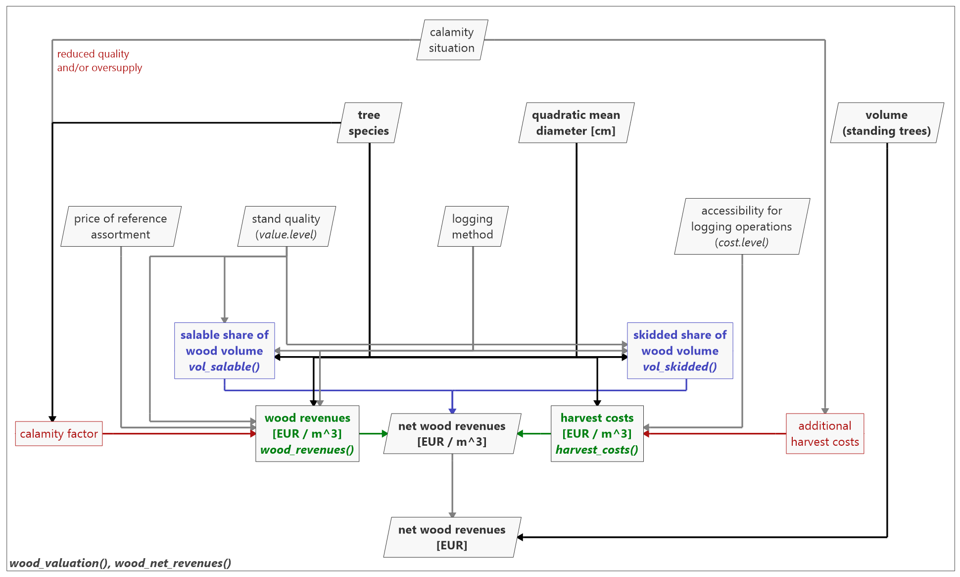
The wood valuation implemented in woodValuationDE is a three-stage approach, deriving (i) the relevant harvest quantities, (ii) the revenues and costs per volume unit, and (iii) the net revenues (see Fig. 1).
woodValuationDE allows for the estimation of
wood values referring to the volume over bark of the standing trees to
be harvested (German unit: Vfm m.R.) as usually provided by yield tables
and single-tree simulation models. Volume losses due to harvest cuts and
residues (in German: X-Holz and NVD-Holz), e.g., due to fixed assortment
length, are considered via the harvest quantity functions:
vol_salable() provides the share
of salable volume relative to the volume over bark. It represents the
volume that is utilized and taken out of the forest stand. It is the
relevant volume unit for the revenues. It includes all pulpwood,
sawlogs, and private fuel wood.
vol_skidded() provides the share
of skidded volume relative to the volume over bark. This volume share is
delivered to the forest road and represents the relevant volume unit for
remuneration for the logging (harvesting and skidding), i.e. the harvest
costs. The salable volume is higher than the skidded volume since it
also includes the private fuel wood, which is not delivered to the
forest road by the forest enterprise.
Accordingly, wood_revenues() estimates the revenues per cubic meter of salable wood [EUR m-3] and harvest_costs() the harvest costs per cubic meter of skidded wood [EUR m-3]. Both models depend on the tree species and quadratic mean diameter3 of the harvested trees. Further function arguments are the stand quality, the logging method, and the accessibility of the stand for logging operations. In addition, current market situations can be considered via updated prices for the German reference assortments.
The functions wood_valuation() and wood_net_revenues() provide wrappers for easy application of the wood valuation procedure implemented in woodValuationDE. Both functions call the previously described ones and combine them to derive the net wood revenues. While wood_valuation() returns a tibble with the entire calculations, wood_net_revenues() can be used to directly get the total net revenues [EUR].
In the next section, we describe the functions’ input arguments and output values as well as the underlying models and data with their references in more detail. The parameters for all models are stored as internal object params.wood.value. Users interested in the detailed parameters can call them via:
woodValuationDE:::params.wood.value3The mean diameter is calculated as the diameter corresponding to the mean single-tree basal area (at breast height) of the harvested trees, often referred to as QMD, Dq, or Dg (see e.g. Curtis and Mashall (2000)). In German: Durchmesser des Grundflächenmittelstamms.
The function estimates the salable share in the volume over bark of the standing trees that are to be harvested. This includes pulpwood, sawlogs, but also private fuel wood. It represents the entire share of wood which is taken out of the forest for usage. The share of salable wood is required to derive the wood revenues per unit volume over bark. The function is based on the assortment tables from Offer and Staupendahl (2018) and its derivation is described in Fuchs et al. (2023). The underlying assortment tables are based on data from HessenForst, the public forest service of the Federal State of Hesse in Germany.
The assortment tables from Offer and Staupendahl (2018) provide conversion factors from the volume over bark (in German: Vfm m.R.) to the harvested volume under bark (in German: Efm o.R.). In addition, they provide the share of non-utilized wood, e.g., due to fixed assortment lengths, and private fuel wood thereof. The assortment tables were derived for HessenForst with the calculation program HOLZERNTE 7.1 (Schöpfer et al., 2003). Additional parameters were defined by forest district officers and validated against harvest and sale statistics of HessenForst. More details on the assortment tables and their derivation are provided in Offer and Staupendahl (2008) and Offer and Staupendahl (2009).
We derived the share of salable volume vsalable based on these assortment tables. Since the assortment tables only provide the values in diameter steps of 2 cm, a Gompertz function was fitted in order to have a continuous model (see Fuchs et al., 2023). For the model fitting, the modified formulation according to Fischer and Schönfelder (2017) was used:
vsalable = A * exp( -exp( zm / A * exp(1) * (tw - dq))),
with the volume share of salable wood vsalable, the quadratic mean diameter dq, and the parameters A, zm and tw. The actual parameter values depend on tree species, stand quality, and logging method.
Apart from species.code.type, all user inputs can be provided as single values or as a vector. If mixed, the single values will be recycled.
The quadratic mean3 of the diameter at breast height (dbh) of the harvested trees [cm].
The tree species, using one of the available species.code.types. Tab. 1 lists the most important genera and species implemented. Most species are assigned to economic species groups for valuation. A list of available species codes and their assignments to economic valuation groups is provided by:
get_species_codes()Tab. 1: Most important species codes and genera available in woodValuationDE with their English and Lower Saxony species codes.
| Species code Lower Saxony | English species Code | Scientific name |
|---|---|---|
| 110 | oak | Quercus sp. |
| 211 | beech | Fagus sylvatica |
| 221 | hornbeam | Carpinus betulus |
| 311 | ash | Fraxinus excelsior |
| 321 | maple | Acer pseudoplatanus |
| 331 | elm | Ulmus glabra |
| 341 | lime | Tilia platyphyllos |
| 354 | cherry | Prunus avium |
| 410 | birch | Betula sp. |
| 421 | alder | Alnus glutinosa |
| 430 | poplar | Populus sp. |
| 441 | willow | Salix sp. |
| 511 | spruce | Picea abies |
| 521 | fir | Abies alba |
| 611 | douglas.fir | Pseudotsuga menziesii |
| 711 | pine | Pinus sylvestris |
| 811 | larch | Larix decidua |
Stand quality, expressed as an integer value of 1:3:
The value.levels refer to the applied assortment tables (Offer and Staupendahl, 2018).
Logging method:
The logging methods “manually” and “harvester” refer to Offer and Staupendahl (2018) and v. Bodelschwingh (2018). Since, e.g., for deciduous species a maximum diameter of 40 cm is assumed for highly mechanized logging, Fuchs et al. (2023) derived the method “combined”. This refers to combinations, as applied by v. Bodelschwingh (2018) in the harvest cost model, assuming diameter-specific proportions of motor-manual and highly mechanized logging:
The type of code in which species is given.
The list with the available species’ codes is provided by:
get_species_codes()A vector with relative shares of salable wood volume (relative share, not percentages).
vol_salable(40,
            "beech")

# species codes Lower Saxony (Germany)
vol_salable(40,
            211,
            species.code.type = "nds")

# vector input
vol_salable(seq(20, 50, 5),
            "spruce")

vol_salable(rep(seq(20, 50, 10),
                2),
            rep(c("beech", "spruce"),
                each = 4))

vol_salable(rep(seq(20, 50, 10),
                2),
            rep(c("beech", "spruce"),
                each = 4),
            logging.method = rep(c("manually", "harvester"),
each = 4))The function estimates the skidded share in the volume over bark of the standing trees that are to be harvested. It is entire volume that is assumed to be commercially delivered to the forest road, the pulpwood and sawlog assortments. The share of skidded wood is required to derive the harvest costs per unit volume over bark. The function is based on the assortment tables from Offer and Staupendahl (2018) and its derivation is described in Fuchs et al. (2023). The underlying assortment tables are based on data from HessenForst, the public forest service of the Federal State of Hesse in Germany.
The assortment tables from Offer and Staupendahl (2018) provide conversion factors from volume over bark to harvested volume under bark. In addition, they provide the share of non-utilized wood, e.g., due to fixed assortment lengths, and private fuelwood thereof. The assortment tables were derived for HessenForst with the calculation program HOLZERNTE 7.1 (Schöpfer et al., 2003). Additional parameters were defined by forest district officers and validated against harvest and sale statistics of HessenForst. More details on the assortment tables and their derivation are provided in Offer and Staupendahl (2008) and Offer and Staupendahl (2009).
We derived the share of skidded volume vskidded based on these assortment tables. Since the assortment tables only provide the values in diameter steps of 2 cm, a Gompertz function was fitted to have a continuous model (see Fuchs et al., 2023). For the model fitting, the modified formulation according to Fischer and Schönfelder (2017) was used:
vskidded = A * exp( -exp( zm / A * exp(1) * (tw - dq))),
with the volume share of skidded wood vskidded, the quadratic mean diameter dq, and the parameters A, zm and tw. The actual parameter values depend on species, stand quality, and logging method.
Apart from species.code.type, all user inputs can be provided as single values or as a vector. If mixed, the single values will be recycled.
For details see vol_salable().
A vector with relative shares of skidded wood volume (relative share, not percentages).
vol_skidded(40,
            "beech")

# species codes Lower Saxony (Germany)
vol_skidded(40,
            211,
            species.code.type = "nds")

# vector input
vol_skidded(seq(20, 50, 5),
            "spruce")

vol_skidded(rep(seq(20, 50, 10),
                2),
            rep(c("beech", "spruce"),
                each = 4))

vol_skidded(rep(seq(20, 50, 10),
                2),
            rep(c("beech", "spruce"),
                each = 4),
            logging.method = rep(c("manually", "harvester"),
each = 4))The function estimates volume shares of specific assortment (groups). These are expressed in relation to the salable volume. At the moment, we implemented the share of saw logs. This also allows for calculating the share of pulp wood. The function is based on the assortment tables from Offer and Staupendahl (2018). Its derivation is similar to the approach described in Fuchs et al. (2023) for the salable and skidded volume. The underlying assortment tables are based on data from HessenForst, the public forest service of the Federal State of Hesse in Germany.
The assortment tables from Offer and Staupendahl (2018) provide conversion factors from volume over bark to harvested volume under bark. In addition, they provide the share of non-utilized wood, e.g., due to fixed assortment lengths, and private fuelwood thereof. The assortment tables were derived for HessenForst with the calculation program HOLZERNTE 7.1 (Schöpfer et al., 2003). Additional parameters were defined by forest district officers and validated against harvest and sale statistics of HessenForst. More details on the assortment tables and their derivation are provided in Offer and Staupendahl (2008) and Offer and Staupendahl (2009).
We derived the share of saw logs vsaw.logs based on these assortment tables. Since the assortment tables only provide the values in diameter steps of 2 cm, a Gompertz function was fitted to have a continuous model (cf. Fuchs et al., 2023). For the model fitting, the modified formulation according to Fischer and Schönfelder (2017) was used:
vsaw.logs = A * exp( -exp( zm / A * exp(1) * (tw - dq))),
with the volume share of saw logs vsaw.logs, the quadratic mean diameter dq, and the parameters A, zm and tw. The actual parameter values depend on species, stand quality, and logging method.
Apart from species.code.type and assortment, all user inputs can be provided as single values or as a vector. If mixed, the single values will be recycled.
Wood assortment whose share is sought, currently implemented: “saw.logs”.
For details see vol_salable().
A vector with relative shares of respective assortment.
# saw log volume per cubic meter salable volume
share.saw.logs <- vol_assortment(40,
                                 "beech",
                                 "saw.logs")
share.saw.logs

# fuel wood per cubic meter salable volume
share.fuel.wood <- (vol_salable(40,
                                "beech") -
                      vol_skidded(40,
                                  "beech")) /
   vol_salable(40,
               "beech")
share.fuel.wood

# pulp wood per cubic meter salable volume
share.pulp.wood <- 1 - share.saw.logs - share.fuel.wood

# saw log volume per cubic meter volume over bark
vol_assortment(40,
               "beech",
               "saw.logs") *
   vol_salable(40,
"beech")The function estimates average wood revenues per unit salable volume [EUR m-3] applying the wood revenues model of v. Bodelschwingh (2018), which is based on the assortment tables from Offer and Staupendahl (2018). Consequences of calamities are implemented based on Dieter (2001), Möllmann and Möhring (2017), Fuchs et al. (2022a), and Fuchs et al. (2022b). Apart from Dieter (2001) and Möllmann and Möhring (2017), the function and all factors are based on data from HessenForst, the public forest service of the Federal State of Hesse in Germany.
The diameter- and species-sensitive wood revenue model was developed by v. Bodelschwingh (2018). It is based on a previous version (2013) of the assortment tables of Offer and Staupendahl (2018) and the wood sales of HessenForst from 2010 to 2015. A price matrix for different assortments was derived out of the sales data and combined with the assortment table to derive average wood revenues for diameter-dependent assortment compositions. The fitted model function for the wood revenues s is:
s = a * dq4 + b * dq3 + c * dq2 + d * dq + e,
with the quadratic mean diameter dq, and the parameters a to e. The parameter values depend on species, stand quality (value.level), and logging method.
The model estimates wood revenues referring to Hessian market conditions in the time period from 2010 to 2015. Via the market price of a reference assortment for each species, this can be linearly adapted to other market conditions. The reference assortments (sawlogs) are defined by diameter class (1: 10-19 cm, 2: 20-29…, with 1a: 10-14 cm and 1b: 15-19 cm) and a quality from A to D (with A the highest and D the lowest quality) as usually applied in Germany (see Deutscher Forstwirtschaftsrat and Deutscher Holzwirtschaftsrat, 2020). The original prices of the reference assortments preference.assortment,original in Hesse between 2010 and 2015 are listed in Tab.2. If another price preference.assortment,user is applied to wood_revenues(), the baseline wood revenues of the model soriginal will be updated (supdated) by:
supdated = preference.assortment,user / preference.assortment,original * soriginal.
Tab. 2: Prices of the reference assortments in Hesse between 2010 and 2015, adapted from v. Bodelschwingh (2018, Tab. 10).
| English Species Code | Reference Assortment | Price [EUR m-3] |
|---|---|---|
| oak | B 4 | 277.41 |
| beech | B 4 | 75.75 |
| spruce | B 2b | 92.47 |
| pine | B 2b | 71.48 |
| douglas.fir | B 2b | 92.23 |
| larch | B 2b | 83.29 |
| birch | B 4 | 72.13 |
| alder | B 4 | 98.90 |
| ash | B 4 | 112.88 |
| poplar | B 4 | 45.43 |
A particular strength of woodValuationDE is the possibility to consider consequences of disturbances and calamities. Users can choose a suitable parameterization from a broad set of previously published estimates for the consequences of disturbances that are pre-implemented. Alternatively, users can implement their own assumptions. For wood revenues, a factor is multiplied with the undisturbed revenues. The options that are implemented by default are listed in Tab. 3.
Tab. 3: Factors to reduce wood revenues for salvage harvests that are implemented in woodValuationDE.
| Name | Factor softwood | Factor deciduous | Reference | Details |
|---|---|---|---|---|
| “none” | 1.00 | 1.00 | - | default: no calamity |
| “calamity.dieter.2001” | 0.50 | 0.50 | Dieter (2001) | Assumption based on prices in southern Germany after a calamity event, often applied in bioeconomic simulations for Germany. Originally referring to net revenues, thus to be used in combination with harvest_costs(). |
| “fire.small.moellmann.2017” | 0.56 | - | Möllmann and Möhring (2017) | Based on a survey of forest managers in Germany, referring to damages by fire affecting only a few trees. The survey only asked for effects of quality losses. |
| “fire.large.moellmann.2017” | 0.56 | - | Möllmann and Möhring (2017) | Based on a survey of forest managers in Germany, referring to damages by fire affecting at least one compartment. The survey only asked for effects of quality losses. |
| “storm.small.moellmann.2017” | 0.85 | 0.79 | Möllmann and Möhring (2017) | Based on a survey of forest managers in Germany, referring to damages by storm affecting only a few trees. The survey only asked for effects of quality losses. |
| “storm.large.moellmann.2017” | 0.85 | 0.79 | Möllmann and Möhring (2017) | Based on a survey of forest managers in Germany, referring to damages by storm affecting at least one compartment. The survey only asked for effects of quality losses. |
| “insects.moellmann.2017” | 0.78 | - | Möllmann and Möhring (2017) | Based on a survey of forest managers in Germany, referring to damages by insects. The survey only asked for effects of quality losses. |
| “ips.fuchs.2022a” | 0.67 | - | Fuchs et al. (2022a) | Assumption of quality losses after spruce bark beetle infestations, based on the assortment tables (Offer and Staupendahl, 2018) and price matrix (v. Bodelschwingh, 2018). |
| “ips.timely.fuchs.2022a” | 0.88 | - | Fuchs et al. (2022a) | Assumption of quality losses after spruce bark beetle infestations with timely salvage harvests leading to lower value losses, based on the assortment tables (Offer and Staupendahl, 2018) and price matrix (v. Bodelschwingh, 2018). |
| “stand.damage.fuchs.2022b” | 0.90 | 0.85 | Fuchs et al. (2022b) | Assumption of damages in a single stand influencing only the wood quality not the wood market, derived based on time series analyses of sales of HessenForst. |
| “regional.disturbance.fuchs.2022b” | 0.74 | 0.70 | Fuchs et al. (2022b) | Assumption of regional damages influencing wood quality and regional wood market (oversupply), derived based on time series analyses of sales of HessenForst. |
| “transregional.calamity.fuchs.2022b” | 0.54 | 0.70 | Fuchs et al. (2022b) | Assumption of (inter-)national damages influencing wood quality and wood national market (oversupply), derived based on time series analyses of sales of HessenForst. |
Apart from species.code.type, price.ref.assortment, and calamity.factors, all user inputs can be provided as single values or as a vector. If mixed, the single values will be recycled.
The quadratic mean3 of the diameter at breast height (dbh) of the harvested trees [cm].
The tree species, using one of the available species.code.types. Tab. 1 lists the most important genera and species implemented. Most species are assigned to economic species groups for valuation. A list of available species codes, and their assignments to valuation groups is provided by:
get_species_codes()Stand quality, expressed as an integer value of 1:3:
The value.levels refer to the applied assortment tables (Offer and Staupendahl, 2018).
Logging method:
The logging methods “manually” and “harvester” refer to Offer and Staupendahl (2018) and v. Bodelschwingh (2018). Since, e.g., for deciduous species a maximum diameter of 40 cm is assumed for highly mechanized logging, Fuchs et al. (2023) derived the method “combined”. This refers to combinations, as applied by v. Bodelschwingh (2018) in the harvest cost model, assuming diameter-specific proportions of motor-manual and highly mechanized logging:
Wood price of the reference assortments allowing for the consideration of market fluctuations as described above. Default is “baseline”, which refers to the prices from 2010 to 2015 in Hesse, Germany according to v. Bodelschwingh (2018), listed in Tab. 2. Alternatively, users can provide a tibble with the same structure, which is illustrated by the “baseline” tibble:
prices.ref.assortments <- dplyr::tibble(
      species = c(110, 211, 511, 711, 611,
                  811, 410, 421, 311, 430),
      price.ref.assortment = c(277.41, 75.75, 92.47, 71.48, 92.23,
83.29, 72.13, 98.90, 112.88, 45.43))Type of calamity or disturbance event in case of salvage harvests. This determines the applied reductions for salvage revenues. For the implemented options, see Tab.3. Alternatively, users can provide their own factors.
Summands [EUR m-3] and factors to consider the consequences of disturbances and calamities on wood revenues and harvest costs. “baseline” provides a tibble based on the references listed in Tab. 5. Alternatively, users can provide an own tibble with the same structure, which is illustrated by the “baseline” tibble:
calamity.factors <- dplyr::tibble(
      calamity.type = rep(c("none",
                            "calamity.dieter.2001",
                            "fire.small.moellmann.2017",
                            "fire.large.moellmann.2017",
                            "storm.small.moellmann.2017",
                            "storm.large.moellmann.2017",
                            "insects.moellmann.2017",
                            "ips.fuchs.2022a",
                            "ips.timely.fuchs.2022a",
                            "stand.damage.fuchs.2022b",
                            "regional.disturbance.fuchs.2022b",
                            "transregional.calamity.fuchs.2022b"),
                          each = 2),
      species.group = rep(c("softwood",
                            "deciduous"),
                          times = 12),
      revenues.factor = c(1.00, 1.00,
                          0.50, 0.50,
                          0.56,   NA,
                          0.56,   NA,
                          0.85, 0.79,
                          0.85, 0.79,
                          0.78,   NA,
                          0.67,   NA,
                          0.88,   NA,
                          0.90, 0.85,
                          0.74, 0.70,
                          0.54, 0.70),
      cost.factor = c(1.00, 1.00,
                      0.50, 0.50,
                      1.17,   NA,
                      1.09,   NA,
                      1.21, 1.24,
                      1.10, 1.12,
                        NA,   NA,
                      1.00,   NA,
                      1.00,   NA,
                      1.15, 1.15,
                      1.15, 1.15,
                      1.25, 1.25),
      cost.additional = c(0.0, 0.0,
                          0.0, 0.0,
                          0.0, 0.0,
                          0.0, 0.0,
                          0.0, 0.0,
                          0.0, 0.0,
                          0.0, 0.0,
                          2.5,  NA,
                          7.5,  NA,
                          0.0, 0.0,
                          0.0, 0.0,
                          0.0, 0.0)
)The type of code in which species is given.
The list with the available species’ codes is provided by:
get_species_codes()A vector with wood revenues per unit volume [EUR m-3]. The volume refers to the share of salable wood volume, which is provided by vol_salable().
wood_revenues(40,
              "beech")

# species codes Lower Saxony (Germany)
wood_revenues(40,
              211,
              species.code.type = "nds")

# vector input
wood_revenues(seq(20, 50, 5),
              "spruce")

wood_revenues(40,
              rep(c("beech", "spruce"),
                  each = 3),
              value.level = rep(1:3, 2))

# with calamity
wood_revenues(40,
              rep("spruce", 7),
              calamity.type = c("none",
                                "calamity.dieter.2001",
                                "ips.fuchs.2022a",
                                "ips.timely.fuchs.2022a",
                                "stand.damage.fuchs.2022b",
                                "regional.disturbance.fuchs.2022b",
                                "transregional.calamity.fuchs.2022b"))

# user-defined calamities with respective changes in wood revenues
wood_revenues(40,
              rep("spruce", 3),
              calamity.type = c("none",
                                "my.own.calamity.1",
                                "my.own.calamity.2"),
              calamity.factors = dplyr::tibble(
                calamity.type = rep(c("none",
                                      "my.own.calamity.1",
                                      "my.own.calamity.2"),
                                    each = 2),
                species.group = rep(c("softwood",
                                      "deciduous"),
                                    times = 3),
                revenues.factor = c(1.0, 1.0,
                                    0.8, 0.8,
                                    0.2, 0.2),
                cost.factor = c(1.0, 1.0,
                                1.5, 1.5,
                                1.0, 1.0),
                cost.additional = c(0, 0,
                                    0, 0,
                                    5, 5)))

# adapted market situation by providing alternative prices for the reference assortments
wood_revenues(40,
              c("oak", "beech", "spruce"))
wood_revenues(40,
              c("oak", "beech", "spruce"),
              price.ref.assortment = dplyr::tibble(
                species = c("oak", "beech", "spruce"),
price.ref.assortment = c(300, 80, 50)))The function estimates harvest costs per unit skidded volume [EUR m-3] applying the harvest costs model of v. Bodelschwingh (2018). Consequences of calamities are implemented based on Dieter (2001), Möllmann and Möhring (2017), Fuchs et al. (2022a), and Fuchs et al. (2022b).
The diameter- and species-sensitive harvest cost model was developed by v. Bodelschwingh (2018). It is based on data from KWF (2006) and AFL (2014). The fitted model function for the harvest costs h is:
h = min(a * dqb + c, hmax),
with the quadratic mean diameter dq, the parameters a to c, and the maximum costs hmax. The parameter values depend on the species and the stand’s accessibility for logging operations (cost.level). The harvest costs were derived for a smaller number of economic species group. The species assignments differ from those for wood_revenues(). The species assignments are provided by:
get_species_codes()The harvest costs are calculated under the assumption of combinations of logging methods, dependent on the quadratic mean of the tree diameters as well as the accessibility of the stand. The accessibility is considered in three cost levels (see Tab. 4). To avoid unusually high harvest costs at smaller diameters, v. Bodelschwingh (2018, Tab. 10) defined maximum harvest costs cmax (see Tab. 4).
Tab. 4: Definitions of the harvest cost levels based on the accessibility of the stand and maximum harvest costs, adapted from v. Bodelschwingh (2018, Tab. 10).
| cost.level | Definition | Maximum Harvest Costs [EUR m-3] |
|---|---|---|
| 3 | slope > 58 % | 80 |
| 2 | slope between 36 % and 58 % AND/OR moist sites | 70 |
| 1 | all other stands without special limitations | 60 |
A special strength of woodValuationDE is the consideration of consequences of disturbances and large-scale calamities. A broad set of previously published and newly derived quantitative effects of calamities is implemented. Additionally, users can implement their own assumptions. For the harvest costs, multiplicative factors as well as absolute summands can be used for implementing consequences of disturbances. The options that are implemented by default are listed in Tab. 5.
Tab. 5: Factors and summands for the consideration of higher harvest costs in case of salvage harvests after disturbances or large-scale calamities, implemented in woodValuationDE.
| Name | Cost Factor Softwood | Additional Costs Softwood [EUR m-3] | Cost Factor Deciduous | Additional Costs Deciduous [EUR m-3] | Reference | Details |
|---|---|---|---|---|---|---|
| “none” | 1.00 | 0.00 | 1.00 | 0.00 | - | default: no calamity |
| “calamity.dieter.2001” | 0.50 | 0.00 | 0.50 | 0.00 | Dieter (2001) | Dieter (2001) assumed a reduction of the net revenues by 0.5 in case of calamities. In our model, this factor is therefore applied to reduce both wood revenues and harvest costs. Obviously this is counterintuitive for the harvest costs and thus to be used in combination with wood_revenues(). |
| “fire.small.moellmann.2017” | 1.17 | 0.00 | NA | NA | Möllmann and Möhring (2017) | Based on a survey of forest managers in Germany, referring to damages by fire affecting only a few trees. |
| “fire.large.moellmann.2017” | 1.09 | 0.00 | NA | NA | Möllmann and Möhring (2017) | Based on a survey of forest managers in Germany, referring to damages by fire affecting at least one compartment. |
| “storm.small.moellmann.2017” | 1.21 | 0.00 | 1.24 | 0.00 | Möllmann and Möhring (2017) | Based on a survey of forest managers in Germany, referring to damages by storm affecting only a few trees. |
| “storm.large.moellmann.2017” | 1.10 | 0.00 | 1.12 | 0.00 | Möllmann and Möhring (2017) | Based on a survey of forest managers in Germany, referring to damages by storm affecting at least one compartment. |
| “insects.moellmann.2017” | NA | NA | NA | NA | Möllmann and Möhring (2017) | Based on a survey of forest managers in Germany, referring to damages by insects. |
| “ips.fuchs.2022a” | 1.00 | 2.50 | NA | NA | Fuchs et al. (2022a) | Assumption of higher harvest costs due to smaller, scattered logging operations. |
| “ips.timely.fuchs.2022a” | 1.00 | 7.50 | NA | NA | Fuchs et al. (2022a) | Assumption of higher harvest costs due to smaller, scattered logging operations, but also including costs for debarking or chemically treating the logs afterwards. |
| “stand.damage.fuchs.2022b” | 1.15 | 0 | 1.15 | 0 | Fuchs et al. (2022b) | Assumption for damages in a single stand with smaller harvest volumes based on experience of HessenForst. |
| “regional.disturbance.fuchs.2022b” | 1.15 | 0 | 1.15 | 0 | Fuchs et al. (2022b) | Assumption for regional damages with smaller harvest volumes based on experience of HessenForst. |
| “transregional.calamity.fuchs.2022b” | 1.25 | 0 | 1.25 | 0 | Fuchs et al. (2022b) | Assumption for transregional damages with smaller harvest volumes and a high demand for timely harvest capacities, based on experience of HessenForst. |
Apart from species.code.type, price.ref.assortment, and calamity.factors, all user inputs can be provided as single values or as a vector. If mixed, the single values will be recycled.
The quadratic mean3 of the diameter at breast height (dbh) of the harvested trees [cm].
The tree species, using one of the available species.code.types. Tab. 1 lists the most important genera and species implemented. Most species are assigned to economic species groups for valuation. A list of available species codes, and their assignments to valuation groups is provided by:
get_species_codes()Accessibility of the stand for logging operations expressed as an integer of 1:3, with 1 for standard conditions without limitations, 2 for moist sites or sites with a slope between 36 % and 58 %, and 3 for slopes > 58 %. The cost.levels refer to the harvest cost model by v. Bodelschwingh (2018, Tab. 10). See also Tab. 4
Type of calamity or disturbance event in case of salvage harvests. This determines the assumption on the increase in harvest costs for salvage harvests. For the implemented options, see Tab.5. Alternatively, users can provide their own assumptions.
Summands [EUR m-3] and factors to consider the consequences of disturbances and calamities on wood revenues and harvest costs. “baseline” provides a tibble based on the references listed in Tab. 5. Alternatively, users can provide an own tibble with the same structure, which is illustrated by the “baseline” tibble:
calamity.factors <- dplyr::tibble(
      calamity.type = rep(c("none",
                            "calamity.dieter.2001",
                            "fire.small.moellmann.2017",
                            "fire.large.moellmann.2017",
                            "storm.small.moellmann.2017",
                            "storm.large.moellmann.2017",
                            "insects.moellmann.2017",
                            "ips.fuchs.2022a",
                            "ips.timely.fuchs.2022a",
                            "stand.damage.fuchs.2022b",
                            "regional.disturbance.fuchs.2022b",
                            "transregional.calamity.fuchs.2022b"),
                          each = 2),
      species.group = rep(c("softwood",
                            "deciduous"),
                          times = 12),
      revenues.factor = c(1.00, 1.00,
                          0.50, 0.50,
                          0.56,   NA,
                          0.56,   NA,
                          0.85, 0.79,
                          0.85, 0.79,
                          0.78,   NA,
                          0.67,   NA,
                          0.88,   NA,
                          0.90, 0.85,
                          0.74, 0.70,
                          0.54, 0.70),
      cost.factor = c(1.00, 1.00,
                      0.50, 0.50,
                      1.17,   NA,
                      1.09,   NA,
                      1.21, 1.24,
                      1.10, 1.12,
                        NA,   NA,
                      1.00,   NA,
                      1.00,   NA,
                      1.15, 1.15,
                      1.15, 1.15,
                      1.25, 1.25),
      cost.additional = c(0.0, 0.0,
                          0.0, 0.0,
                          0.0, 0.0,
                          0.0, 0.0,
                          0.0, 0.0,
                          0.0, 0.0,
                          0.0, 0.0,
                          2.5,  NA,
                          7.5,  NA,
                          0.0, 0.0,
                          0.0, 0.0,
                          0.0, 0.0)
)The type of code in which species is given.
The list with the available species codes is provided by:
get_species_codes()A vector with harvest costs per unit volume [EUR m-3]. The volume refers to the share of skidded wood volume, provided by vol_skidded().
harvest_costs(40,
              "beech")

# species codes Lower Saxony (Germany)
harvest_costs(40,
              211,
              species.code.type = "nds")

# vector input
harvest_costs(seq(20, 50, 5),
              "spruce")

harvest_costs(40,
              rep(c("beech", "spruce"),
                  each = 3),
              cost.level = rep(1:3, 2))

harvest_costs(40,
              rep("spruce", 6),
              calamity.type = c("none",
                                "calamity.dieter.2001",
                                "ips.fuchs.2022a",
                                "ips.timely.fuchs.2022a",
                                "stand.damage.fuchs.2022b",
                                "regional.disturbance.fuchs.2022b",
                                "transregional.calamity.fuchs.2022b"))

# user-defined calamities with respective changes in harvest costs
harvest_costs(40,
              rep("spruce", 3),
              calamity.type = c("none",
                                "my.own.calamity.1",
                                "my.own.calamity.2"),
              calamity.factors = dplyr::tibble(
                calamity.type = rep(c("none",
                                      "my.own.calamity.1",
                                      "my.own.calamity.2"),
                                    each = 2),
                species.group = rep(c("softwood",
                                      "deciduous"),
                                    times = 3),
                revenues.factor = c(1.0, 1.0,
                                    0.8, 0.8,
                                    0.2, 0.2),
                cost.factor = c(1.0, 1.0,
                                1.5, 1.5,
                                1.0, 1.0),
                cost.additional = c(0, 0,
                                    0, 0,
5, 5)))The function is a wrapper for the entire procedure of wood valuation implemented in woodValuationDE. It estimates the share of salable (for revenues) and skidded volume (for harvest costs) as well as the wood revenues and harvest costs per unit volume. Finally, it derives the net revenues for the user-provided volume (referring to the volume over bark).
The function applies the previously described models implemented in the functions vol_salable(), vol_skidded(), wood_revenues(), and harvest_costs().
Wood volume [m3], referring to volume over bark of the trees to be harvested (German unit Vfm m.R.) as usually provided by yield tables and single-tree simulation models.
The quadratic mean3 of the diameter at breast height (dbh) of the harvested trees [cm].
The tree species, using one of the available species.code.types. Tab. 1 lists the most important genera and species implemented. Most species are assigned to economic species groups for valuation. A list of available species codes, and their assignments to valuation groups is provided by:
get_species_codes()Stand quality, expressed as an integer value of 1:3:
The value.levels refer to the applied assortment tables (Offer and Staupendahl, 2018).
Accessibility of the stand for logging operations expressed as an integer of 1:3, with 1 for standard conditions without limitations, 2 for moist sites or sites with a slope between 36 % and 58 %, and 3 for slopes > 58 %. The cost.levels refer to the harvest cost model by v. Bodelschwingh (2018, Tab. 10). See also Tab. 4
Logging method:
The logging methods “manually” and “harvester” refer to Offer and Staupendahl (2018) and v. Bodelschwingh (2018). Since, e.g., for deciduous species a maximum diameter of 40 cm is assumed for highly mechanized logging, Fuchs et al. (2023) derived the method “combined”. This refers to combinations, as applied by v. Bodelschwingh (2018) in the harvest cost model, assuming diameter-specific proportions of motor-manual and highly mechanized logging:
Wood price of the reference assortments allowing for the consideration of market fluctuations. Default is “baseline”, which refers to the prices from 2010 to 2015 in Hesse, Germany according to v. Bodelschwingh (2018), listed in Tab. 2. Alternatively, users can provide a tibble with the same structure, which is illustrated by the “baseline” tibble:
prices.ref.assortments <- dplyr::tibble(
      species = c(110, 211, 511, 711, 611,
                  811, 410, 421, 311, 430),
      price.ref.assortment = c(277.41, 75.75, 92.47, 71.48, 92.23,
83.29, 72.13, 98.90, 112.88, 45.43))Type of calamity or disturbance event in case of salvage harvests. This determines the applied reductions for salvage revenues. For the implemented options, see Tab.3. Alternatively, users can provide their own factors.
Summands [EUR m-3] and factors to consider the consequences of disturbances and calamities on wood revenues and harvest costs. “baseline” provides a tibble based on the references listed in Tab. 5. Alternatively, users can provide an own tibble with the same structure, which is illustrated by the “baseline” tibble:
calamity.factors <- dplyr::tibble(
      calamity.type = rep(c("none",
                            "calamity.dieter.2001",
                            "fire.small.moellmann.2017",
                            "fire.large.moellmann.2017",
                            "storm.small.moellmann.2017",
                            "storm.large.moellmann.2017",
                            "insects.moellmann.2017",
                            "ips.fuchs.2022a",
                            "ips.timely.fuchs.2022a",
                            "stand.damage.fuchs.2022b",
                            "regional.disturbance.fuchs.2022b",
                            "transregional.calamity.fuchs.2022b"),
                          each = 2),
      species.group = rep(c("softwood",
                            "deciduous"),
                          times = 12),
      revenues.factor = c(1.00, 1.00,
                          0.50, 0.50,
                          0.56,   NA,
                          0.56,   NA,
                          0.85, 0.79,
                          0.85, 0.79,
                          0.78,   NA,
                          0.67,   NA,
                          0.88,   NA,
                          0.90, 0.85,
                          0.74, 0.70,
                          0.54, 0.70),
      cost.factor = c(1.00, 1.00,
                      0.50, 0.50,
                      1.17,   NA,
                      1.09,   NA,
                      1.21, 1.24,
                      1.10, 1.12,
                        NA,   NA,
                      1.00,   NA,
                      1.00,   NA,
                      1.15, 1.15,
                      1.15, 1.15,
                      1.25, 1.25),
      cost.additional = c(0.0, 0.0,
                          0.0, 0.0,
                          0.0, 0.0,
                          0.0, 0.0,
                          0.0, 0.0,
                          0.0, 0.0,
                          0.0, 0.0,
                          2.5,  NA,
                          7.5,  NA,
                          0.0, 0.0,
                          0.0, 0.0,
                          0.0, 0.0)
)The type of code in which species is given.
The list with the available species’ codes is provided by:
get_species_codes()A tibble with all steps of the wood valuation (harvest quantities, harvest costs per unit skidded volume [EUR m-3], wood revenues per unit salable volume [EUR m-3], and total net revenues [EUR]).
wood_valuation(1,
               40,
               "beech")

# species codes Lower Saxony (Germany)
wood_valuation(seq(10, 70, 20),
               40,
               211,
               species.code.type = "nds")

# vector input
wood_valuation(10,
               seq(20, 50, 5),
               "spruce")

wood_valuation(10,
               40,
               rep(c("beech", "spruce"),
                   each = 9),
               value.level = rep(rep(1:3, 2),
                                 each = 3),
               cost.level = rep(1:3, 6))

wood_valuation(10,
               40,
               rep("spruce", 6),
               calamity.type = c("none",
                                 "ips.fuchs.2022a",
                                 "ips.timely.fuchs.2022a",
                                 "stand.damage.fuchs.2022b",
                                 "regional.disturbance.fuchs.2022b",
                                 "transregional.calamity.fuchs.2022b"))

# user-defined calamities with respective changes in harvest costs and wood revenues
wood_valuation(10,
               40,
               rep("spruce", 3),
               calamity.type = c("none",
                                 "my.own.calamity.1",
                                 "my.own.calamity.2"),
               calamity.factors = dplyr::tibble(
                 calamity.type = rep(c("none",
                                       "my.own.calamity.1",
                                       "my.own.calamity.2"),
                                     each = 2),
                 species.group = rep(c("softwood",
                                       "deciduous"),
                                     times = 3),
                 revenues.factor = c(1.0, 1.0,
                                     0.8, 0.8,
                                     0.2, 0.2),
                 cost.factor = c(1.0, 1.0,
                                 1.5, 1.5,
                                 1.0, 1.0),
                 cost.additional = c(0, 0,
                                     0, 0,
                                     5, 5)))

# adapted market situation by providing alternative prices for the reference assortments
wood_valuation(10,
               40,
               c("oak", "beech", "spruce"))
wood_valuation(10,
               40,
               c("oak", "beech", "spruce"),
               price.ref.assortment = dplyr::tibble(
                 species = c("oak", "beech", "spruce"),
price.ref.assortment = c(300, 80, 50)))The function is a wrapper for the wood valuation provided by woodValuationDE. It calls wood_valuation() and returns only the net revenues for the user-provided volume referring to the volume over bark.
The function applies the previously described models implemented in the functions vol_salable(), vol_skidded(), wood_revenues(), and harvest_costs().
Wood volume [m3], referring to volume over bark of the trees to be harvested (German unit Vfm m.R.) as usually provided by yield tables and single-tree simulation models.
The quadratic mean3 of the diameter at breast height (dbh) of the harvested trees [cm].
The tree species, using one of the available species.code.types. Tab. 1 lists the most important genera and species implemented. Most species are assigned to economic species groups for valuation. A list of available species codes, and their assignments to valuation groups is provided by:
get_species_codes()Stand quality, expressed as an integer value of 1:3:
The value.levels refer to the applied assortment tables (Offer and Staupendahl, 2018).
Accessibility of the stand for logging operations expressed as an integer of 1:3, with 1 for standard conditions without limitations, 2 for moist sites or sites with a slope between 36 % and 58 %, and 3 for slopes > 58 %. The cost.levels refer to the harvest cost model by v. Bodelschwingh (2018, Tab. 10). See also Tab. 4
Logging methods:
The logging methods “manually” and “harvester” refer to Offer and Staupendahl (2018) and v. Bodelschwingh (2018). Since, e.g., for deciduous species a maximum diameter of 40 cm is assumed for highly mechanized logging, Fuchs et al. (2023) derived the method “combined”. This refers to combinations, as applied by v. Bodelschwingh (2018) in the harvest cost model, assuming diameter-specific proportions of motor-manual and highly mechanized logging:
Wood price of the reference assortments allowing for the consideration of market fluctuations. Default is “baseline”, which refers to the prices from 2010 to 2015 in Hesse, Germany according to v. Bodelschwingh (2018), listed in Tab. 2. Alternatively, users can provide a tibble with the same structure, which is illustrated by the “baseline” tibble:
prices.ref.assortments <- dplyr::tibble(
      species = c(110, 211, 511, 711, 611,
                  811, 410, 421, 311, 430),
      price.ref.assortment = c(277.41, 75.75, 92.47, 71.48, 92.23,
83.29, 72.13, 98.90, 112.88, 45.43))Type of calamity or disturbance event in case of salvage harvests. This determines the applied reductions for salvage revenues. For the implemented options, see Tab.3. Alternatively, users can provide their own factors.
Summands [EUR m-3] and factors to consider the consequences of disturbances and calamities on wood revenues and harvest costs. “baseline” provides a tibble based on the references listed in Tab. 5. Alternatively, users can provide an own tibble with the same structure, which is illustrated by the “baseline” tibble:
calamity.factors <- dplyr::tibble(
      calamity.type = rep(c("none",
                            "calamity.dieter.2001",
                            "fire.small.moellmann.2017",
                            "fire.large.moellmann.2017",
                            "storm.small.moellmann.2017",
                            "storm.large.moellmann.2017",
                            "insects.moellmann.2017",
                            "ips.fuchs.2022a",
                            "ips.timely.fuchs.2022a",
                            "stand.damage.fuchs.2022b",
                            "regional.disturbance.fuchs.2022b",
                            "transregional.calamity.fuchs.2022b"),
                          each = 2),
      species.group = rep(c("softwood",
                            "deciduous"),
                          times = 12),
      revenues.factor = c(1.00, 1.00,
                          0.50, 0.50,
                          0.56,   NA,
                          0.56,   NA,
                          0.85, 0.79,
                          0.85, 0.79,
                          0.78,   NA,
                          0.67,   NA,
                          0.88,   NA,
                          0.90, 0.85,
                          0.74, 0.70,
                          0.54, 0.70),
      cost.factor = c(1.00, 1.00,
                      0.50, 0.50,
                      1.17,   NA,
                      1.09,   NA,
                      1.21, 1.24,
                      1.10, 1.12,
                        NA,   NA,
                      1.00,   NA,
                      1.00,   NA,
                      1.15, 1.15,
                      1.15, 1.15,
                      1.25, 1.25),
      cost.additional = c(0.0, 0.0,
                          0.0, 0.0,
                          0.0, 0.0,
                          0.0, 0.0,
                          0.0, 0.0,
                          0.0, 0.0,
                          0.0, 0.0,
                          2.5,  NA,
                          7.5,  NA,
                          0.0, 0.0,
                          0.0, 0.0,
                          0.0, 0.0)
)The type of code in which species is given.
The list with the available species’ codes is provided by:
get_species_codes()A vector with the total net revenues for the volume over bark of the trees to be harvested [EUR].
wood_net_revenues(1,
                  40,
                  "beech")

# species codes Lower Saxony (Germany)
wood_net_revenues(seq(10, 70, 20),
                  40,
                  211,
                  species.code.type = "nds")

# vector input
wood_net_revenues(10,
                  seq(20, 50, 5),
                  "spruce")

wood_net_revenues(10,
                  40,
                  rep(c("beech", "spruce"),
                      each = 9),
                  value.level = rep(rep(1:3, 2),
                                    each = 3),
                  cost.level = rep(1:3, 6))

wood_net_revenues(10,
                  40,
                  rep("spruce", 6),
                  calamity.type = c("none",
                                    "calamity.dieter.2001",
                                    "ips.fuchs.2022a",
                                    "ips.timely.fuchs.2022a",
                                    "stand.damage.fuchs.2022b",
                                    "regional.disturbance.fuchs.2022b",
                                    "transregional.calamity.fuchs.2022b"))

# user-defined calamities with respective changes in harvest costs and wood revenues
wood_net_revenues(10,
                  40,
                  rep("spruce", 3),
                  calamity.type = c("none",
                                    "my.own.calamity.1",
                                    "my.own.calamity.2"),
                  calamity.factors = dplyr::tibble(
                    calamity.type = rep(c("none",
                                          "my.own.calamity.1",
                                          "my.own.calamity.2"),
                                        each = 2),
                    species.group = rep(c("softwood",
                                          "deciduous"),
                                        times = 3),
                    revenues.factor = c(1.0, 1.0,
                                        0.8, 0.8,
                                        0.2, 0.2),
                    cost.factor = c(1.0, 1.0,
                                    1.5, 1.5,
                                    1.0, 1.0),
                    cost.additional = c(0, 0,
                                        0, 0,
                                        5, 5)))

# adapted market situation by providing alternative prices for the reference assortments
wood_net_revenues(10,
                  40,
                  c("oak", "beech", "spruce"))
wood_net_revenues(10,
                  40,
                  c("oak", "beech", "spruce"),
                  price.ref.assortment = dplyr::tibble(
                    species = c("oak", "beech", "spruce"),
price.ref.assortment = c(300, 80, 50)))The function returns all available species, species codes, and species assignments to groups for the economic valuation.
A list with the available species, species codes, and their assignments to economic species groups.
get_species_codes()In the following, we will demonstrate the application of woodValuationDE using yield tables. We will show the calculations required to obtain the figures presented below. These are similar to those included in the technical note (Fuchs et al., 2023). In contrast to the technical note, we use the new generation of yield tables (Nuske et al., 2022) as an example for a growth model.
First, we install woodValuationDE. We load the required R packages, including the et.nwfva package (Nuske et al., 2022) that provides yield table data for our example:
install.packages("woodValuationDE")

library(woodValuationDE)
library(tidyverse)
library(readxl)
library(ggplot2)
library(patchwork)
library(et.nwfva)
We then import the yield tables:
yield.table <-  bind_rows(
  tibble(species = "oak",
         et_tafel(art = c("Eiche"),
                  bon = -1,
                  bon_typ = "relativ")),
  tibble(species = "beech",
         et_tafel(art = c("Buche"),
                  bon = -1,
                  bon_typ = "relativ")),
  tibble(species = "spruce",
         et_tafel(art = c("Fichte"),
                  bon = -1,
                  bon_typ = "relativ")),
  tibble(species = "douglas.fir",
         et_tafel(art = c("Douglasie"),
                  bon = -1,
                  bon_typ = "relativ")),
  tibble(species = "pine",
         et_tafel(art = c("Kiefer"),
                  bon = -1,
                  bon_typ = "relativ"))
)

yield.table <- yield.table %>%
  select(species,
         h.100.m = H100,
         age = Alter,
         diameter.remaining.cm = Dg,
         volume.remaining.m3.ha = V)
We add some information and translations for the visualization.
species.list <- tibble(
  en = c("beech",
         "douglas.fir",
         "oak",
         "spruce",
         "pine"),
  de = c("Buche",
         "Douglasie",
         "Eiche",
         "Fichte",
         "Kiefer"))

# plotted mean diameters [cm]
diameter.range <- c(10, 60)

# colors tree species (Lower Saxony)
colors <- c(
  "oak"         = rgb(255, 255,   0, maxColorValue = 255),
  "beech"       = rgb(189,  91,  57, maxColorValue = 255),
  "spruce"      = rgb(  0, 200, 255, maxColorValue = 255),
  "douglas.fir" = rgb(255,   0, 255, maxColorValue = 255),
  "pine"        = rgb(191, 191, 191, maxColorValue = 255)
)
Calculate harvest quantities, revenues, and costs over the diameter range specified above. The functions are applied with default parameters for the five species available in the yield tables.
dat.1 <- tibble(
  species = rep(
    species.list$en,
    each = length(seq(diameter.range[1],
                      diameter.range[2],
                      0.1))),
  diameter = rep(
    seq(diameter.range[1],
        diameter.range[2],
        0.1),
    times = nrow(species.list))
) %>%
  mutate(
    skidded.volume = vol_skidded(
      diameter,
      species),
    salable.volume = vol_salable(
      diameter,
      species),
    harvest.costs = harvest_costs(
      diameter,
      species),
    wood.revenues = wood_revenues(
      diameter,
      species),
    wood.net.revenues = wood_net_revenues(
      1, # 1 m^3
      diameter,
      species)

  )

# long format for plotting
dat.1.gath <- dat.1 %>%
  gather("variable",
         "value",
         -species,
         -diameter) %>%
  # reasonable order in the plot
  mutate(variable = factor(variable,
                           levels = c("salable.volume",
                                      "skidded.volume",
                                      "harvest.costs",
                                      "wood.revenues",
                                      "wood.net.revenues")))
Harvest quantities:
p1.1 <-
  ggplot() +
  geom_hline(yintercept = 0,
             col = "grey40",
             linetype = "dashed") +
  geom_line(
    data = filter(dat.1.gath,
                  variable %in% c("skidded.volume",
                                  "salable.volume")),
    aes(diameter,
        value,
        col = species),
    linewidth = 1) +
  labs(x = "Quadratic mean diameter [cm]",
       y = "Relative volume share") +
  scale_x_continuous(breaks = seq(10, 60, 10)) +
  scale_color_manual(values = colors) +
  theme_bw() +
  theme(legend.position = "none") +
  facet_wrap(~variable)
Revenues and costs:
p1.2 <-
  ggplot() +
  geom_hline(yintercept = 0,
             col = "grey40",
             linetype = "dashed") +
  geom_line(
    data = filter(dat.1.gath,
                  variable %in% c("harvest.costs",
                                  "wood.revenues",
                                  "wood.net.revenues")),
    aes(diameter,
        value,
        color = species),
    linewidth = 1) +
  labs(x = "Quadratic mean diameter [cm]",
       y = bquote("Costs or (net) revenues [\u20AC m"^-3~"]")) +
  scale_x_continuous(breaks = seq(10, 60, 10)) +
  scale_color_manual(values = colors) +
  theme_bw() +
  theme(legend.position = "bottom") +
  facet_wrap(~variable)
Combined plot:
p1.1 / p1.2 + plot_annotation(tag_levels = "a")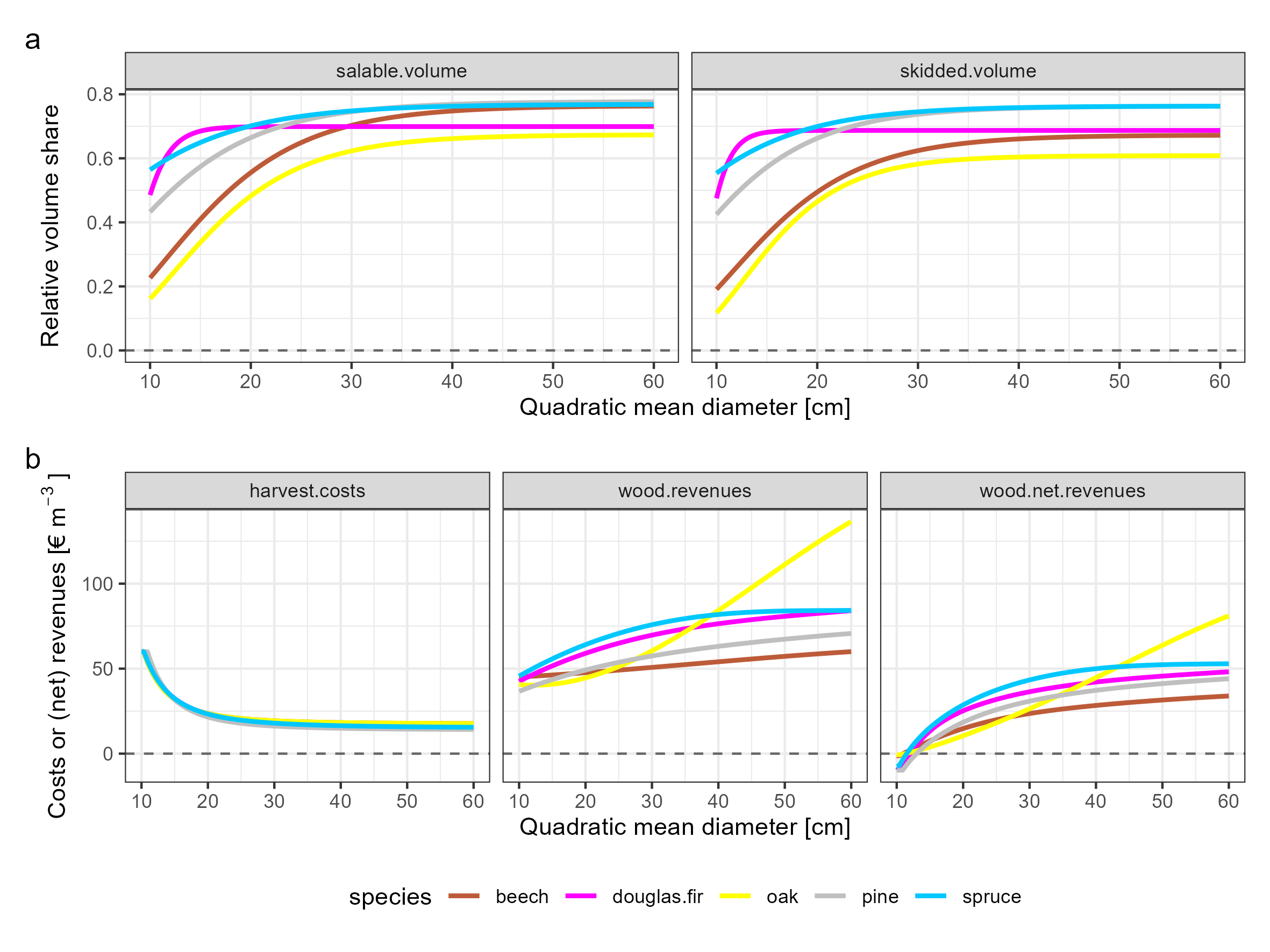
For this figure, we calculate stumpage values over age based on the yield tables. The figure should illustrate the influence of the stand quality (value level) as well as the accessibility for harvest operations (cost level).
dat.2 <- yield.table %>%
  filter(diameter.remaining.cm <= 60 &
           diameter.remaining.cm >= 10)

dat.2a <- dat.2[rep(1:nrow(dat.2),
                    times = 9), ] %>%
  add_column(value.level = rep(1:3,
                               each = nrow(dat.2) * 3)) %>%
  add_column(cost.level = rep(rep(1:3,
                                  each = nrow(dat.2)),
                              times = 3)) %>%
  mutate(
    net.revenue = wood_net_revenues(
      volume = volume.remaining.m3.ha,
      diameter.q = diameter.remaining.cm,
      species = species,
      value.level = value.level,
      cost.level = cost.level))

# fixed cost level for the influence of the stand quality
dat.2.1 <- dat.2a %>%
  filter(cost.level == 1)

# fixed value level for the influence of the accessibility
dat.2.2 <- dat.2a %>%
  filter(value.level == 2)
Influence of the stand quality:
p2.1 <- ggplot() +
  geom_hline(yintercept = 0,
             col = "grey40",
             linetype = "dashed") +
  geom_line(data = dat.2.1,
            aes(age,
                net.revenue,
                col = as.factor(value.level)),
            linewidth = 1) +
  scale_x_continuous(breaks = c(seq(40, 160, 40))) +
  scale_color_discrete(name = "value.level") +
  labs(x = "Age [a]",
       y = bquote("Net stumpage value [\u20AC ha"^-1~"]")) +
  theme_bw() +
  theme(legend.position = "bottom") +
  facet_wrap(~species)
Influence of the accessibility for harvest operations:
p2.2 <- ggplot() +
  geom_hline(yintercept = 0,
             col = "grey40",
             linetype = "dashed") +
  geom_line(data = dat.2.2,
            aes(age,
                net.revenue,
                col = as.factor(cost.level)),
            linewidth = 1) +
  scale_x_continuous(breaks = c(seq(40, 160, 40))) +
  scale_color_discrete(name = "cost.level") +
  labs(x = "Age [a]",
       y = bquote("Net stumpage value [\u20AC ha"^-1~"]")) +
  theme_bw() +
  theme(legend.position = "bottom") +
  facet_wrap(~species)
Combined plot:
p2.1 + p2.2 +
  plot_layout(nrow = 2) +
  plot_annotation(tag_levels = "a")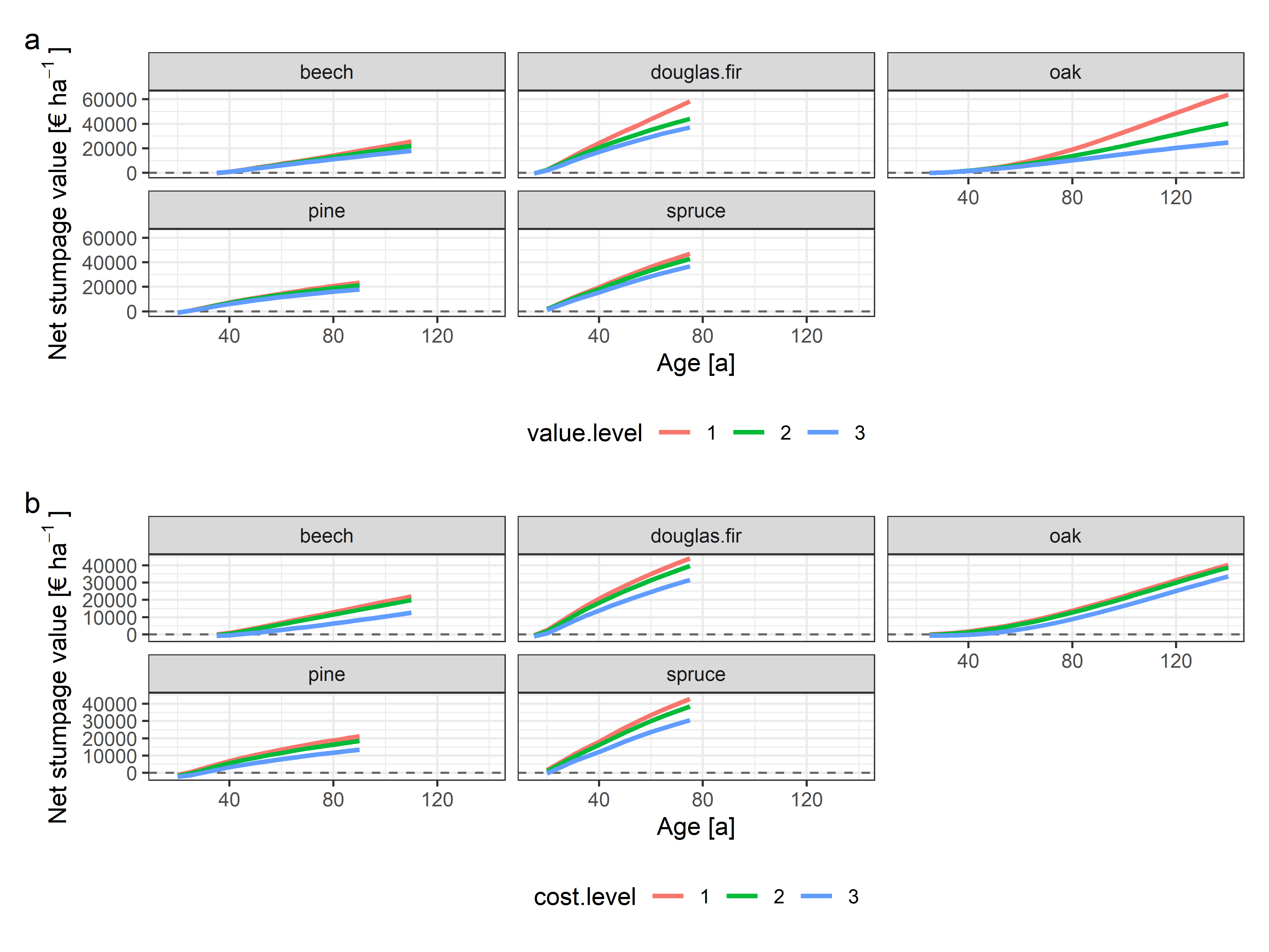
This figure illustrates the different assumptions on the consequences of calamities that we implemented in our package. We compare stumpage values of spruce and beech stands (age 70) without disturbances (“none”) and with the different assumptions on reductions in revenues and increases in costs in the case of a salvage harvest.
dat.3 <- yield.table %>%
  filter(species %in% c("beech",
                        "spruce")) %>%
  filter(age == 70)

dat.3a <- dat.3[rep(1:2,
                    times = 11), ] %>%
  mutate(
    calamity.reference = rep(
      c("transregional.calamity.fuchs.2022b",
        "regional.disturbance.fuchs.2022b",
        "stand.damage.fuchs.2022b",
        "ips.timely.fuchs.2022a",
        "ips.fuchs.2022a",
        "fire.large.moellmann.2017",
        "fire.small.moellmann.2017",
        "storm.large.moellmann.2017",
        "storm.small.moellmann.2017",
        "calamity.dieter.2001",
        "none"),
      each = 2),
    net.stumpage.value =
      wood_net_revenues(
        volume = volume.remaining.m3.ha,
        diameter.q = diameter.remaining.cm,
        species = species,
        calamity.type = calamity.reference
      ),
    calamity.reference = as_factor(calamity.reference)
  )
You will receive three warnings. 1+3: Some assumptions on the consequences of calamities apply only to coniferous species. Thus, the function returns NA values for beech. 2: Please note that Dieter (2001) assumed a reduction in net revenues by a factor of 0.5. Thus, the revenues and costs are only meaningful if they are interpreted in their sum (as net revenues).
Plot:
ggplot() +
  geom_hline(yintercept = 0,
             col = "gray60") +
  geom_hline(data = filter(dat.3a,
                           calamity.reference == "none"),
             aes(yintercept = net.stumpage.value),
             linetype = "dashed",
             col = "gray40") +
  geom_bar(data = dat.3a,
           aes(calamity.reference,
               net.stumpage.value,
               fill = calamity.reference),
           stat = "identity") +
  labs(x = "Calamity type",
       y = bquote("Net stumpage value [\u20AC ha"^-1~"]")) +
  theme_bw() +
  theme(legend.position = "none") +
  coord_flip() +
  facet_wrap(~species,
             ncol = 1)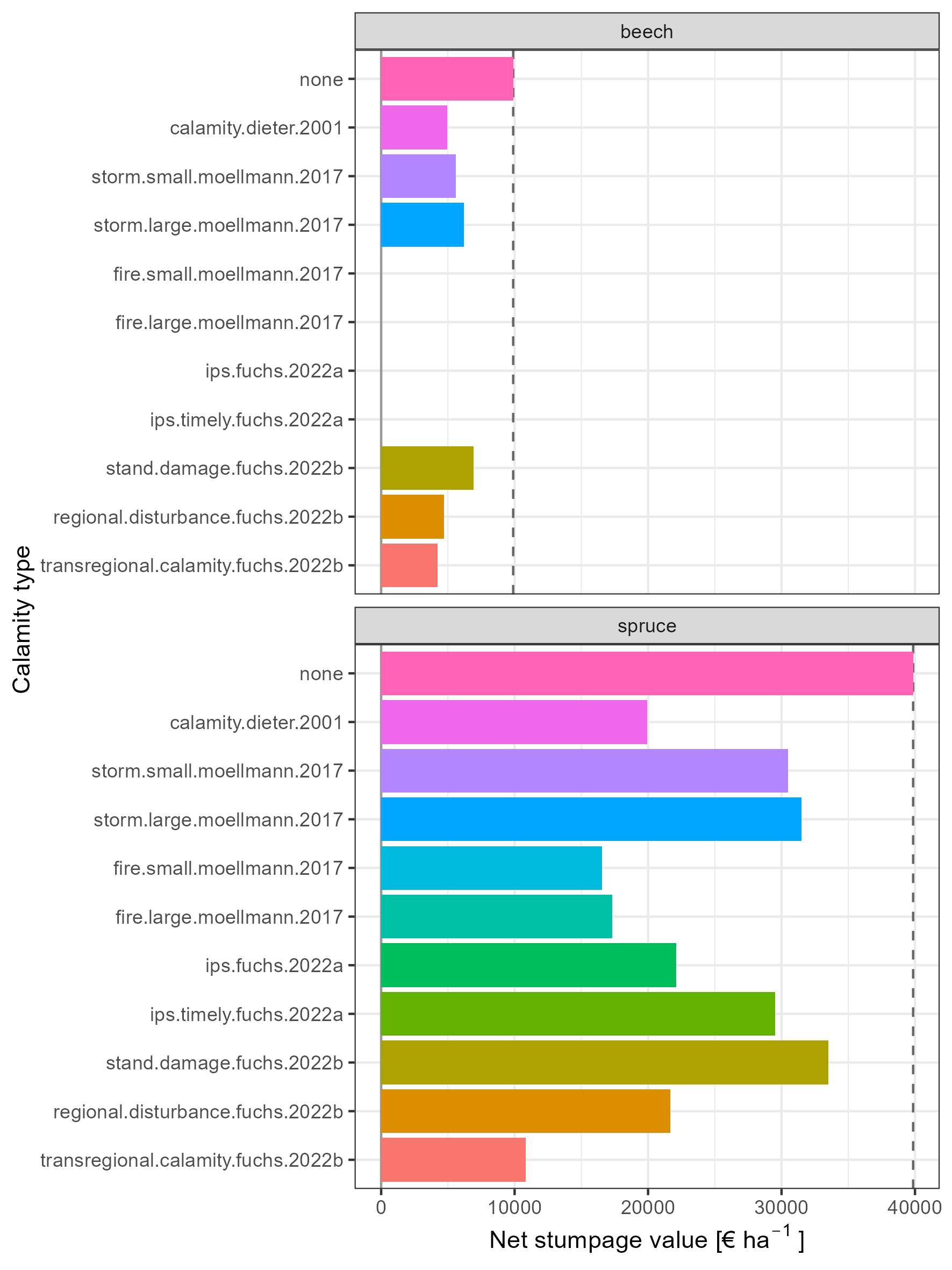
Fuchs, Jasper M.; Husmann, Kai; v. Bodelschwingh, Hilmar; Koster, Roman; Staupendahl, Kai; Offer, Armin; Möhring, Bernhard; Paul, Carola (2023): woodValuationDE: A consistent framework for calculating stumpage values in Germany (technical note). Allg. Forst- u. J.-Ztg. 193 (1/2), p. 16-29. doi: 10.23765/afjz0002090.
Bibtex:
@article{
  title = {{{woodValuationDE}}: {{A}} Consistent Framework for Calculating Stumpage Values in {{Germany}} (Technical Note)},
  author = {Fuchs, Jasper M. and Husmann, Kai and {von Bodelschwingh}, Hilmar and Koster, Roman and Staupendahl, Kai and Offer, Armin and M{\"o}hring, Bernhard and Paul, Carola},
  year = {2023},
  journal = {Allg. Forst- Jagdztg.},
  volume = {193},
  number = {1/2},
  pages = {16--29},
  doi = {10.23765/afjz0002090}
}
For details on the applied models and underlying assumptions, such as assumptions on the economic consequences of disturbances, please also cite the original publication(s).
This work is part of a PhD project by J.F., partly financed by the University of Göttingen and supported by the Graduate School Forest and Agricultural Sciences Göttingen. J.F. further acknowledges partial funding through the Federal Ministry of Education and Research Germany (BMBF) in the 2019-2020 BiodivERsA joint call for research proposals, under the BiodivClim ERA-Net COFUND programme, and with the funding organisations Academy of Finland (decision no. 344722), ANR (France, project ANR-20-EBI5-0005-03), and Federal Ministry of Education and Research (Germany, grant no. 16LC2021A).
AfL (ed.) (2014): AfL-Info 2014/15. Richtpreise, Tarife, Kalkulationen, Adressen. [Reference prices, tariffs, calculations, addresses]. AfL Niedersachsen e.V. Hannover: Deutscher Landwirtschaftsverlag.
Curtis, Robert O.; Marshall, David D. (2000): Technical Note: Why Quadratic Mean Diameter? West. J. Appl. For. 15 (3), p. 137-139. https://doi.org/10.1093/wjaf/15.3.137.
Deutscher Forstwirtschaftsrat e.V.; Deutscher Holzwirtschaftsrat e.V. (2020): Rahmenvereinbarung für den Rohholzhandel in Deutschland (RVR). [Master Agreement for Raw Wood Trading in Germany]. 3rd ed. Fachagentur Nachwachsende Rohstoffe e.V. (FNR). Gülzow-Prüzen. Online available at https://www.fnr.de/fileadmin/kiwuh/broschueren/Broschuere_RVR2020_Nachdruck_web.pdf.
Dieter, Matthias (2001): Land expectation values for spruce and beech calculated with Monte Carlo modelling techniques. For. Policy Econ. 2 (2), p. 157-166. https://doi.org/10.1016/S1389-9341(01)00045-4.
Fischer, Christoph; Schönfelder, Egbert (2017): A modified growth function with interpretable parameters applied to the age–height relationship of individual trees. Can. J. For. Res. 47, p. 166–173. https://doi.org/10.1139/cjfr-2016-0317.
Fuchs, Jasper M.; Hittenbeck, Anika; Brandl, Susanne; Schmidt, Matthias; Paul, Carola (2022b): Adaptation Strategies for Spruce Forests - Economic Potential of Bark Beetle Management and Douglas Fir Cultivation in Future Tree Species Portfolios. Forestry 95 (2), p. 229-246. https://doi.org/10.1093/forestry/cpab040
Fuchs, Jasper M.; v. Bodelschwingh, Hilmar; Paul, Carola; Husmann, Kai (2022a): Quantifying the consequences of disturbances on wood revenues with Impulse Response Functions. For. Policy Econ. 140, art. 102738. https://doi.org/10.1016/j.forpol.2022.102738.
Fuchs, Jasper M.; Husmann, Kai; v. Bodelschwingh, Hilmar; Koster, Roman; Staupendahl, Kai; Offer, Armin; Möhring, Bernhard; Paul, Carola (2023): woodValuationDE: A consistent framework for calculating stumpage values in Germany (technical note). Allg. Forst- u. J.-Ztg. 193 (1/2), p. 16-29. doi: 10.23765/afjz0002090.
KWF (ed.) (2006): Holzernteverfahren - Vergleichende Erhebung und Beurteilung, Daten CD mit Beschreibung der Ernteverfahren und Kalkulationen. [Wood harvesting methods - Comparative survey and assessment, data CD with description of harvesting methods and calculations.]. Groß-Umstadt: KWF.
Möllmann, Torsten B.; Möhring, Bernhard (2017): A practical way to integrate risk in forest management decisions. Ann. For. Sci. 74 (4), p. 75-87. https://doi.org/10.1007/s13595-017-0670-x.
Nuske, Robert; Staupendahl, Kai; Albert, Matthias (2022). et.nwfva: Forest Yield Tables for Northwest Germany and their Application (Version 0.1.1) [Computer software]. https://github.com/rnuske/et.nwfva and https://CRAN.R-project.org/package=et.nwfva
Offer, Armin; Staupendahl, Kai (2008): Neue Bestandessortentafeln für die Waldbewertung und ihr Einsatz in der Bewertungspraxis. [New stand assortment tables for forest valuation and their application in valuation practice.]. Wertermittlungsforum 26 (4), p. 146-154.
Offer, Armin; Staupendahl, Kai (2009): Neue Bestandessortentafeln für die Waldbewertung und ihr Einsatz in der Bewertungspraxis. [New stand assortment tables for forest valuation and their application in valuation practice.]. Forst und Holz 64 (5), p. 16–25.
Offer, Armin; Staupendahl, Kai (2018): Holzwerbungskosten- und Bestandessortentafeln (Wood Harvest Cost and Assortment Tables). Kassel: HessenForst (publisher).
Schöpfer, W.; Kändler, G.; Stöhr, D. (2003): Entscheidungshilfen für die Forst- und Holzwirtschaft - Zur Abschlussversion von HOLZERNTE. [Decision Support for Forestry and Wood Industry - The Final Version of HOLZERNTE]. Forst und Holz 58 (18), p. 545–550.
v. Bodelschwingh, Hilmar (2018): Oekonomische Potentiale von Waldbeständen. Konzeption und Abschätzung im Rahmen einer Fallstudie in hessischen Staatswaldflächen [Economic Potentials of Forest Stands and Their Consideration in Strategic Decisions]. Bad Orb: J.D. Sauerländer`s Verlag (Schriften zur Forst- und Umweltökonomie, 47).