u5mr![]()
u5mr is a open-source R package for estimating the child
mortality. Current implementation includes the Trussell version of the
Brass method using the Coale-Demeny model life tables and supporting
datasets of coefficients and automatic interpolating values between
probabilities of dying at a certain age and model tables.
To download the developmental version of the u5mr package, use the code below.
# install.packages("devtools")
devtools::install_github("myominnoo/u5mr")The first example is using Bangladesh survey data and model South of the Coale-Demeny life table.
library(u5mr)

## Using Bangladesh survey data to estimate child mortality
data("bangladesh")
bang_both <- u5mr_trussell(bangladesh, sex = "both", model = "south", svy_year = 1974.3)
bang_both
#>   agegrp   women child_born child_dead        pi        di        ki        qx
#> 1  15-19 3014706    1160919     215365 0.3850853 0.1855125 0.9170244 0.1701195
#> 2  20-24 2653155    4901382     997384 1.8473787 0.2034904 0.9954643 0.2025674
#> 3  25-29 2607009    9085852    1937955 3.4851633 0.2132937 0.9906944 0.2113089
#> 4  30-34 2015663    9910256    2261196 4.9166235 0.2281673 1.0075009 0.2298787
#> 5  35-39 1771680   10384001    2490168 5.8611041 0.2398081 1.0293505 0.2468466
#> 6  40-44 1479575    9164329    2415023 6.1938928 0.2635243 1.0094877 0.2660245
#> 7  45-49 1135129    6905673    1959544 6.0836020 0.2837586 0.9972749 0.2829853
#>          ti   year          h        q5
#> 1  1.179512 1973.1 0.06844071 0.2936809
#> 2  2.573340 1971.7 0.69835995 0.2393985
#> 3  4.591300 1969.7 0.25513876 0.2298161
#> 4  6.972056 1967.3 0.25803543 0.2298787
#> 5  9.601908 1964.7 0.22544741 0.2291742
#> 6 12.426746 1961.9 0.60317713 0.2373407
#> 7 15.521768 1958.8 0.68837645 0.2391827
bang_male <- u5mr_trussell(bangladesh, child_born = "male_born",
                 child_dead = "male_dead", sex = "male",
                 model = "south", svy_year = 1974.3)
bang_male
#>   agegrp   women child_born child_dead        pi        di        ki        qx
#> 1  15-19 3014706     597248     117165 0.1981115 0.1961748 0.9105728 0.1786314
#> 2  20-24 2653155    2507018     529877 0.9449195 0.2113575 0.9956980 0.2104482
#> 3  25-29 2607009    4675978    1047294 1.7936179 0.2239733 0.9923244 0.2222541
#> 4  30-34 2015663    5109487    1204582 2.5348915 0.2357540 1.0092759 0.2379408
#> 5  35-39 1771680    5435726    1333957 3.0681195 0.2454055 1.0311249 0.2530437
#> 6  40-44 1479575    4883599    1291745 3.3006769 0.2645068 1.0111377 0.2674528
#> 7  45-49 1135129    3714957    1030737 3.2727179 0.2774560 0.9987376 0.2771057
#>          ti   year          h        q5
#> 1  1.192502 1973.1 0.08877256 0.3006920
#> 2  2.579408 1971.7 0.13536167 0.2555678
#> 3  4.579127 1969.7 0.47824926 0.2412141
#> 4  6.935584 1967.4 0.32705901 0.2379408
#> 5  9.538031 1964.8 0.21974177 0.2356174
#> 6 12.341232 1962.0 0.42457992 0.2400522
#> 7 15.432413 1958.9 0.24483379 0.2361607
bang_female <- u5mr_trussell(bangladesh, child_born = "female_born",
                 child_dead = "female_dead", sex = "female",
                 model = "south", svy_year = 1974.3)
bang_female
#>   agegrp   women child_born child_dead        pi        di        ki        qx
#> 1  15-19 3014706     563671      98200 0.1869738 0.1742151 0.9238170 0.1609429
#> 2  20-24 2653155    2394364     467507 0.9024591 0.1952531 0.9952065 0.1943172
#> 3  25-29 2607009    4409874     890661 1.6915454 0.2019697 0.9889674 0.1997415
#> 4  30-34 2015663    4800769    1056614 2.3817320 0.2200927 1.0056231 0.2213302
#> 5  35-39 1771680    4948275    1156211 2.7929846 0.2336594 1.0274741 0.2400790
#> 6  40-44 1479575    4280730    1123278 2.8932160 0.2624034 1.0077431 0.2644352
#> 7  45-49 1135129    3190716     928807 2.8108840 0.2910967 0.9957282 0.2898532
#>          ti   year          h        q5
#> 1  1.165826 1973.1 0.02505353 0.2857318
#> 2  2.566995 1971.7 0.02066463 0.2394660
#> 3  4.604250 1969.7 0.01367451 0.2177052
#> 4  7.010693 1967.3 0.18157708 0.2213302
#> 5  9.669503 1964.6 0.22027538 0.2221657
#> 6 12.517197 1961.8 0.78201764 0.2342938
#> 7 15.616267 1958.7 0.15543868 0.2425051

## plotting all data points
with(bang_both,
    plot(year, q5, type = "b", pch = 19,
         ylim = c(0, .45),
         col = "black", xlab = "Reference date", ylab = "u5MR",
         main = paste0("Under-Five mortality, q(5) in Bangladesh, estimated\n",
                       "using model South and the Trussell version of the Brass method")))
with(bang_both, text(year, q5, agegrp, cex=0.65, pos=3,col="purple"))
with(bang_male, lines(year, q5, pch = 18, col = "red", type = "b", lty = 2))
with(bang_female,
    lines(year, q5, pch = 18, col = "blue", type = "b", lty = 3))
legend("bottomright", legend=c("Both sexes", "Male", "Female"),
      col = c("Black", "red", "blue"), lty = 1:3, cex=0.8)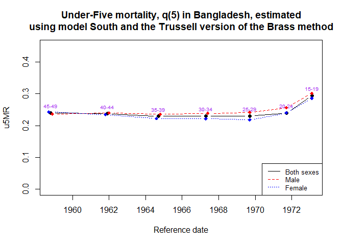
Below, the second example is demonstrated using Panama survey data and model West.
## Using panama survey data to estimate child mortality
data("panama")
pnm_both <- u5mr_trussell(panama, sex = "both", model = "west", svy_year = 1976.5)
pnm_both
#>   agegrp women child_born child_dead       pi         di        ki         qx
#> 1  15-19  2695        557         40 0.206679 0.07181329 1.0664294 0.07658380
#> 2  20-24  2095       2633        130 1.256802 0.04937334 1.0404542 0.05137070
#> 3  25-29  1828       4757        312 2.602298 0.06558756 0.9937778 0.06517946
#> 4  30-34  1605       6085        435 3.791277 0.07148726 1.0041775 0.07178590
#> 5  35-39  1362       6722        636 4.935389 0.09461470 1.0221369 0.09670918
#> 6  40-44  1128       6367        686 5.644504 0.10774305 1.0099799 0.10881831
#> 7  45-49   930       5276        689 5.673118 0.13059136 1.0021669 0.13087434
#>          ti   year          h         q5
#> 1  1.048001 1975.5 0.81948565 0.10681851
#> 2  2.364852 1974.1 0.92645560 0.05824125
#> 3  4.314966 1972.2 0.67558234 0.07022363
#> 4  6.636520 1969.9 0.77255738 0.07178590
#> 5  9.194406 1967.3 0.77689110 0.08856392
#> 6 11.924192 1964.6 0.07458829 0.09364872
#> 7 14.855814 1961.6 0.62026040 0.10329620
pnm_male <- u5mr_trussell(panama, child_born = "male_born",
                child_dead = "male_dead", sex = "male",
                model = "west", svy_year = 1976.5)
pnm_male
#>   agegrp women child_born child_dead        pi         di        ki         qx
#> 1  15-19  2695        278         24 0.1031540 0.08633094 1.1028540 0.09521042
#> 2  20-24  2095       1380         77 0.6587112 0.05579710 1.0394544 0.05799854
#> 3  25-29  1828       2395        172 1.3101751 0.07181628 0.9850075 0.07073958
#> 4  30-34  1605       3097        236 1.9295950 0.07620278 0.9938784 0.07573630
#> 5  35-39  1362       3444        348 2.5286344 0.10104530 1.0109014 0.10214683
#> 6  40-44  1128       3274        394 2.9024823 0.12034209 0.9983923 0.12014862
#> 7  45-49   930       2682        354 2.8838710 0.13199105 0.9908787 0.13078712
#>           ti   year         h         q5
#> 1  0.9648135 1975.5 0.7281892 0.13193006
#> 2  2.3270195 1974.2 0.9840888 0.06559956
#> 3  4.3919097 1972.1 0.6078929 0.07600789
#> 4  6.8621158 1969.6 0.5916396 0.07573630
#> 5  9.5808416 1966.9 0.6441241 0.09378708
#> 6 12.4282225 1964.1 0.2231215 0.10404412
#> 7 15.3637414 1961.1 0.2131179 0.10386235
pnm_female <- u5mr_trussell(panama, child_born = "female_born",
                child_dead = "female_dead", sex = "female",
                model = "west", svy_year = 1976.5)
pnm_female
#>   agegrp women child_born child_dead        pi         di       ki         qx
#> 1  15-19  2695        279         16 0.1035250 0.05734767 1.027639 0.05893272
#> 2  20-24  2095       1253         53 0.5980907 0.04229848 1.041099 0.04403690
#> 3  25-29  1828       2362        140 1.2921225 0.05927180 1.002714 0.05943267
#> 4  30-34  1605       2988        199 1.8616822 0.06659973 1.014781 0.06758414
#> 5  35-39  1362       3278        288 2.4067548 0.08785845 1.033741 0.09082286
#> 6  40-44  1128       3093        292 2.7420213 0.09440672 1.021957 0.09647958
#> 7  45-49   930       2594        335 2.7892473 0.12914418 1.013832 0.13093046
#>          ti   year          h         q5
#> 1  1.136167 1975.4 0.89036801 0.08250300
#> 2  2.407031 1974.1 0.82492745 0.05003973
#> 3  4.238697 1972.3 0.75975955 0.06427108
#> 4  6.406109 1970.1 0.97378159 0.06758414
#> 5  8.796807 1967.7 0.91344410 0.08287914
#> 6 11.404035 1965.1 0.88800323 0.08246445
#> 7 14.331051 1962.2 0.04466646 0.10226980

## plotting all data points
with(pnm_both,
    plot(year, q5, type = "b", pch = 19,
        ylim = c(0, .2), col = "black", xlab = "Reference date", ylab = "u5MR",
         main = paste0("Under-Five mortality, q(5) in Panama, estimated\n",
                       "using model West and the Trussell version of the Brass method")))
with(pnm_both, text(year, q5, agegrp, cex=0.65, pos=3,col="purple"))
with(pnm_male,
    lines(year, q5, pch = 18, col = "red", type = "b", lty = 2))
with(pnm_female,
    lines(year, q5, pch = 18, col = "blue", type = "b", lty = 3))
legend("bottomleft", legend=c("Both sexes", "Male", "Female"),
      col = c("Black", "red", "blue"), lty = 1:3, cex=0.8)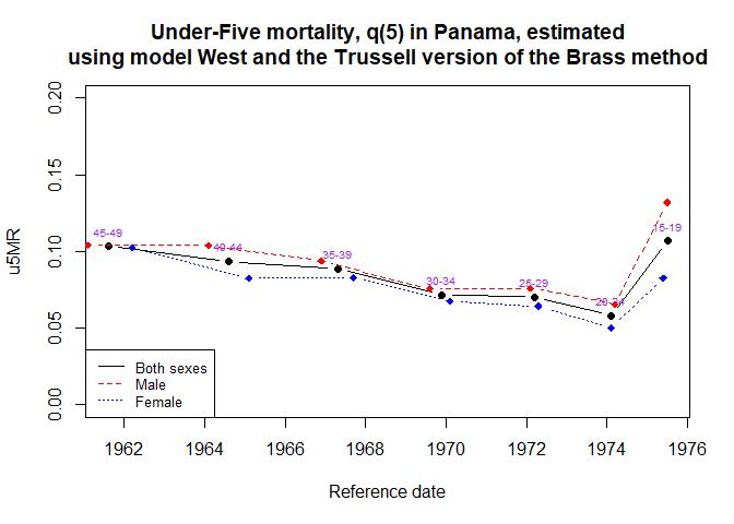
If you encounter a clear bug, please file an issue with a minimal reproducible example on GitHub.
For questions and other discussion, please directly email me dr.myominnoo@gmail.com.
To cite the u5mr package in publications use
  @Manual{Myo2020space,
    title = {Under-Five Child Mortality Estimation using the R Package u5mr},
    author = {Myo Minn Oo},
    year = {2021}
  }
Please note that this project is looking for contributors. By participating in this project, you agree to abide by its terms with Contributor Code of Conduct, version 1.0.0, available at https://www.contributor-covenant.org/version/1/0/0/code-of-conduct/.