![]()
![]()
trendeval aims to provide a coherent interface for evaluating models fit with the trending package. Whilst it is useful in an interactive context, it’s main focus is to provide an intuitive interface on which other packages can be developed (e.g. trendbreaker).
You can install the stable version of this package from CRAN with:
install.packages("trendeval")The development version can be installed from GitHub with:
if (!require(remotes)) {
  install.packages("remotes")
}
remotes::install_github("reconverse/trendeval", build_vignettes = TRUE)library(dplyr) # for data manipulation
library(outbreaks) # for data
#> Warning: package 'outbreaks' was built under R version 4.4.3
library(trending) # for trend fitting
#> Warning: package 'trending' was built under R version 4.4.3
library(trendeval) # for model selection
# load data
data(covid19_england_nhscalls_2020)
# define a selection of model in a named list
models <- list(
simple = lm_model(count ~ day),
glm_poisson = glm_model(count ~ day, family = "poisson"),
glm_poisson_weekday = glm_model(count ~ day + weekday, family = "quasipoisson"),
glm_quasipoisson = glm_model(count ~ day, family = "poisson"),
glm_quasipoisson_weekday = glm_model(count ~ day + weekday, family = "quasipoisson"),
glm_negbin = glm_nb_model(count ~ day),
glm_negbin_weekday = glm_nb_model(count ~ day + weekday),
will_error = glm_nb_model(count ~ day + nonexistant)
)
# select 8 weeks of data (from a period when the prevalence was decreasing)
last_date <- as.Date("2020-05-28")
first_date <- last_date - 8*7
pathways_recent <-
covid19_england_nhscalls_2020 %>%
filter(date >= first_date, date <= last_date) %>%
group_by(date, day, weekday) %>%
summarise(count = sum(count), .groups = "drop")
# split data for fitting and prediction
dat <-
pathways_recent %>%
group_by(date <= first_date + 6*7) %>%
group_split()
fitting_data <- dat[[2]]
pred_data <- select(dat[[1]], date, day, weekday)
# assess the models using the evaluate_resampling
results <-
models %>%
evaluate_resampling(fitting_data, metric = "rmse") %>%
summary
results
#> # A tibble: 8 × 5
#> model_name metric value splits_averaged nas_removed
#> <chr> <chr> <dbl> <dbl> <dbl>
#> 1 glm_negbin rmse 7159. 5 0
#> 2 glm_negbin_weekday rmse 6348. 5 0
#> 3 glm_poisson rmse 7224. 5 0
#> 4 glm_poisson_weekday rmse 6981. 5 0
#> 5 glm_quasipoisson rmse 6819. 5 0
#> 6 glm_quasipoisson_weekday rmse 5924. 5 0
#> 7 simple rmse 9064. 5 0
#> 8 will_error rmse NaN 5 5library(tidyr) # for data manipulation
library(purrr) # for data manipulation
library(ggplot2) # for plotting
#> Warning: package 'ggplot2' was built under R version 4.4.3
# Pull out the model with the lowest RMSE
best_by_rmse <-
results %>%
slice_min(value) %>%
select(model_name) %>%
pluck(1,1) %>%
pluck(models, .)
# Now let's look at the following 14 days as well
new_dat <-
covid19_england_nhscalls_2020 %>%
filter(date > "2020-05-28", date <= "2020-06-11") %>%
group_by(date, day, weekday) %>%
summarise(count = sum(count), .groups = "drop")
all_dat <- bind_rows(pathways_recent, new_dat)
out <-
best_by_rmse %>%
fit(pathways_recent) %>%
predict(all_dat) %>%
pluck(1) %>%
.subset2(1L)
out
#> <trending_prediction> 71 x 9
#> date day weekday count estimate lower_ci upper_ci lower_pi upper_pi
#> <date> <int> <fct> <int> <dbl> <dbl> <dbl> <dbl> <dbl>
#> 1 2020-04-02 15 rest_of_… 71917 58301. 53120. 63988. 40268 79935
#> 2 2020-04-03 16 rest_of_… 63365 56280. 51398. 61625. 38771 77291
#> 3 2020-04-04 17 weekend 52412 47107. 41966. 52878. 30644 67450
#> 4 2020-04-05 18 weekend 54014 45474. 40576. 50962. 29459 65284
#> 5 2020-04-06 19 monday 78996 62206. 54362. 71181. 41350 87955
#> 6 2020-04-07 20 rest_of_… 62026 48871. 45017. 53054. 33258 67650
#> 7 2020-04-08 21 rest_of_… 51692 47176. 43540. 51116. 31991 65458
#> 8 2020-04-09 22 rest_of_… 40797 45540. 42108. 49253. 30765 63346
#> 9 2020-04-10 23 rest_of_… 33946 43961. 40718. 47463. 29580 61313
#> 10 2020-04-11 24 weekend 32269 36796. 33092. 40916. 23141 53834
#> # ℹ 61 more rows
# plot output
ggplot(out, aes(x = date, y = count)) +
geom_line() +
geom_ribbon(mapping = aes(x = date, ymin = lower_ci, ymax = upper_ci),
data = out, alpha = 0.5, fill = "#BBB67E") +
geom_ribbon(mapping = aes(x = date, ymin = lower_pi, ymax = upper_pi),
data = out, alpha = 0.5, fill = "#BBB67E") +
geom_vline(xintercept = as.Date("2020-05-28") + 0.5) +
theme_bw()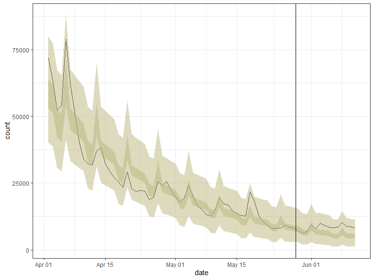
Bug reports and feature requests should be posted on github using the issue system. All other questions should be posted on the RECON slack channel see https://www.repidemicsconsortium.org/forum/ for details on how to join.