A R/MATLAB package to construct and compare single-cell gene regulatory networks (scGRNs) using single-cell RNA-seq (scRNA-seq) data collected from different conditions based on machine learning methods. scTenifoldNet uses principal component regression, tensor decomposition, and manifold alignment, to accurately identify even subtly shifted gene expression programs.
scTenifoldNet is available through the CRAN repositories, you can install scTenifoldNet, using the following command:
install.packages('scTenifoldNet')
library(scTenifoldNet)
Or if you are interested in the version in development, you can install scTenifoldNet, using the following command:
library(remotes)
install_github('cailab-tamu/scTenifoldNet')
library(scTenifoldNet)| Code | Function |
|---|---|
| scQC | Performs single-cell data quality control |
| cpmNormalization | Performs counts per million (CPM) data normalization |
| pcNet | Computes a gene regulatory network based on principal component regression |
| makeNetworks | Computes gene regulatory networks for subsamples of cells based on principal component regression |
| tensorDecomposition | Performs CANDECOMP/PARAFAC (CP) Tensor Decomposition |
| manifoldAlignment | Performs non-linear manifold alignment of two gene regulatory networks |
| dRegulation | Evaluates gene differential regulation based on manifold alignment distances |
| scTenifoldNet | Construct and compare single-cell gene regulatory networks (scGRNs) using single-cell RNA-seq (scRNA-seq) data sets collected from different conditions based on principal component regression, tensor decomposition, and manifold alignment. |
The required input for scTenifoldNet is an expression matrix with genes in the rows and cells (barcodes) in the columns. Data is expected to be not normalized if the main scTenifoldNet function is used. Given the modular structure of the package, users are free to include modifications in each step to perform their analysis.
The running time of scTenifoldNet is largely dependent on how long it takes to construct scGRNs from subsampled expression matrices. Time increases proportional to the number of cells and genes in the dataset used as input. Below is a table of running times under different scenarios:
| Number of Cells | Number of Genes | Running Time |
|---|---|---|
| 300 | 1000 | 3.45 min |
| 1000 | 1000 | 4.25 min |
| 1000 | 5000 | 171.88 min (2 h 51.6 min) |
| 2500 | 5000 | 175.29 min (2 h 55.3 min) |
| 5000 | 5000 | 188.88 min (3 h 8.9 min) |
| 5000 | 7500 | 189.51 min (3 h 9.5 min) |
| 7500 | 5000 | 615.45 min (10 h 15.5 min) |
| 7500 | 7500 | 616.12 min (10 h 16.1 min) |
The output of scTenifoldNet is a list with 3 slots as follows: * tensorNetworks: The computed weight-averaged denoised gene regulatory networks after CANDECOMP/PARAFAC (CP) tensor decomposition. It includes two slots with: * X: The constructed network for the X sample. * Y: The constructed network for the Y sample. * manifoldAlignment: The generated low-dimensional features result of the non-linear manifold alignment. It is a data frame with 2 times the number of genes in the rows and d (default= 30) dimensions in the columns * diffRegulation: The results of the differential regulation analysis. It is a data frame with 6 columns as follows: * gene: A character vector with the gene id identified from the manifoldAlignment output. * distance: A numeric vector of the Euclidean distance computed between the coordinates of the same gene in both conditions. * Z: A numeric vector of the Z-scores computed after Box-Cox power transformation. * FC: A numeric vector of the FC computed with respect to the expectation. * p.value: A numeric vector of the p-values associated to the fold-changes, probabilities are asigned as P[X > x] using the Chi-square distribution with one degree of freedom. * p.adj: A numeric vector of adjusted p-values using Benjamini & Hochberg (1995) FDR correction.
Once installed, scTenifoldNet can be loaded typing:
library(scTenifoldNet)Here we simulate a dataset of 2000 cells (columns) and 100 genes (rows) following the negative binomial distribution with high sparsity (~67%). We label the last ten genes as mitochondrial genes (‘mt-’) to perform single-cell quality control.
nCells = 2000
nGenes = 100
set.seed(1)
X <- rnbinom(n = nGenes * nCells, size = 20, prob = 0.98)
X <- round(X)
X <- matrix(X, ncol = nCells)
rownames(X) <- c(paste0('ng', 1:90), paste0('mt-', 1:10))We generate a perturbed network modifying the expression of genes 10, 2, and 3 and replacing them with the expression of genes 50, 11, and 5.
Y <- X
Y[10,] <- Y[50,]
Y[2,] <- Y[11,]
Y[3,] <- Y[5,]Here we run scTenifoldNet under the H0 (there is no change in the regulation of the gene) using the same matrix as input and under the HA (there is a change in the regulation of the genes) using the control and the perturbed network.
outputH0 <- scTenifoldNet(X = X, Y = X,
                          nc_nNet = 10, nc_nCells = 500,
                          td_K = 3, qc_minLibSize = 30)

outputHA <- scTenifoldNet(X = X, Y = Y,
                          nc_nNet = 10, nc_nCells = 500,
                          td_K = 3, qc_minLibSize = 30)
The output of sctTenifoldNet is a list with 3 slots containing: tensorNetworks: The computed weight-averaged denoised gene regulatory networks after CANDECOMP/PARAFAC (CP) tensor decomposition, manifoldAlignment: The generated low-dimensional features result of the non-linear manifold alignment, and diffRegulation: The results of the differential regulation analysis.
Networks are provided as matrices of class dgCMatrix that can be easily converted into an igraph object as follows: ```{r} # Network for sample X igraph::graph_from_adjacency_matrix(adjmatrix = outputH0\(tensorNetworks\)X, weighted = TRUE) # IGRAPH 28b1d49 DNW- 100 2836 – # + attr: name (v/c), weight (e/n) # + edges from 28b1d49 (vertex names): # [1] ng6 ->ng1 ng12->ng1 ng14->ng1 ng24->ng1 ng28->ng1 ng31->ng1 ng42->ng1 ng44->ng1 ng49->ng1 ng55->ng1 # [11] ng56->ng1 ng59->ng1 ng62->ng1 ng63->ng1 ng72->ng1 ng73->ng1 ng74->ng1 ng77->ng1 ng80->ng1 ng82->ng1 # [21] ng83->ng1 ng87->ng1 ng89->ng1 mt-1->ng1 mt-5->ng1 mt-7->ng1 ng27->ng3 ng28->ng3 ng31->ng3 ng32->ng3 # [31] ng44->ng3 ng59->ng3 ng62->ng3 ng72->ng3 ng73->ng3 ng74->ng3 ng77->ng3 ng82->ng3 ng87->ng3 ng89->ng3 # [41] mt-5->ng3 mt-7->ng3 ng28->ng4 ng59->ng4 ng74->ng4 ng6 ->ng6 ng12->ng6 ng14->ng6 ng16->ng6 ng17->ng6 # [51] ng19->ng6 ng21->ng6 ng23->ng6 ng24->ng6 ng27->ng6 ng28->ng6 ng31->ng6 ng32->ng6 ng33->ng6 ng38->ng6 # [61] ng39->ng6 ng42->ng6 ng46->ng6 ng47->ng6 ng49->ng6 ng51->ng6 ng54->ng6 ng55->ng6 ng56->ng6 ng60->ng6 # [71] ng62->ng6 ng63->ng6 ng65->ng6 ng73->ng6 ng77->ng6 ng78->ng6 ng80->ng6 ng83->ng6 ng86->ng6 mt-1->ng6 # + … omitted several edges
# Network for sample Y igraph::graph_from_adjacency_matrix(outputH0\(tensorNetworks\)Y,weighted = TRUE) # IGRAPH 4b81093 DNW- 100 2836 – # + attr: name (v/c), weight (e/n) # + edges from 4b81093 (vertex names): # [1] ng6 ->ng1 ng12->ng1 ng14->ng1 ng24->ng1 ng28->ng1 ng31->ng1 ng42->ng1 ng44->ng1 ng49->ng1 ng55->ng1 # [11] ng56->ng1 ng59->ng1 ng62->ng1 ng63->ng1 ng72->ng1 ng73->ng1 ng74->ng1 ng77->ng1 ng80->ng1 ng82->ng1 # [21] ng83->ng1 ng87->ng1 ng89->ng1 mt-1->ng1 mt-5->ng1 mt-7->ng1 ng27->ng3 ng28->ng3 ng31->ng3 ng32->ng3 # [31] ng44->ng3 ng59->ng3 ng62->ng3 ng72->ng3 ng73->ng3 ng74->ng3 ng77->ng3 ng82->ng3 ng87->ng3 ng89->ng3 # [41] mt-5->ng3 mt-7->ng3 ng28->ng4 ng59->ng4 ng74->ng4 ng6 ->ng6 ng12->ng6 ng14->ng6 ng16->ng6 ng17->ng6 # [51] ng19->ng6 ng21->ng6 ng23->ng6 ng24->ng6 ng27->ng6 ng28->ng6 ng31->ng6 ng32->ng6 ng33->ng6 ng38->ng6 # [61] ng39->ng6 ng42->ng6 ng46->ng6 ng47->ng6 ng49->ng6 ng51->ng6 ng54->ng6 ng55->ng6 ng56->ng6 ng60->ng6 # [71] ng62->ng6 ng63->ng6 ng65->ng6 ng73->ng6 ng77->ng6 ng78->ng6 ng80->ng6 ng83->ng6 ng86->ng6 mt-1->ng6 # + … omitted several edges ``` igraph provides functions for the topological analysis of biological networks.
The generated low-dimensional features result of the non-linear manifold alignment is reported as an object of class data.frame with 2 times the number of tested genes and d dimensions (by default= 30). The information of the X sample is located at the top of the list followed by the one for the Y sample.
head(outputH0$manifoldAlignment)
#           NLMA 1        NLMA 2        NLMA 3        NLMA 4        NLMA 5        NLMA 6        NLMA 7
# X_ng1  3.455615e-02  3.337002e-03  3.476070e-02  2.643282e-02 -1.425302e-02  1.349180e-02 -1.985468e-02
# X_ng2 -1.863298e-15  2.909680e-15 -7.743151e-18 -1.197043e-14  1.892979e-15 -3.189950e-16 -3.683088e-15
# X_ng3 -2.972715e-02 -1.733728e-02 -1.517115e-02 -6.137618e-03 -2.391348e-03  1.022138e-02  2.340274e-02
# X_ng4  2.865644e-03  4.388924e-03  4.554574e-03 -1.373470e-04 -3.835945e-03  1.063513e-02  8.833412e-03
# X_ng5 -1.646604e-15  2.194729e-15  4.894927e-16 -1.089279e-14  1.154941e-15  1.271950e-15 -1.532357e-15
# X_ng6  7.804296e-02 -1.989693e-01  1.573542e-01 -2.353141e-02 -4.731798e-03  5.829295e-02 -8.294162e-03
#            NLMA 8        NLMA 9       NLMA 10       NLMA 11       NLMA 12       NLMA 13       NLMA 14
# X_ng1  2.635041e-02 -2.345245e-02 -5.703322e-02  1.114734e-01  1.649660e-02 -4.579573e-02  3.471257e-02
# X_ng2  5.097370e-15  1.637280e-14  1.829759e-15 -8.624639e-15 -1.407086e-15 -1.140506e-14 -1.744113e-14
# X_ng3 -1.820885e-03  1.792514e-02  2.575468e-02 -7.237932e-03 -1.614833e-02 -5.961137e-03  2.176211e-02
# X_ng4 -1.664665e-02  1.728433e-03 -3.859241e-03  3.072121e-03 -3.317193e-04 -4.220318e-03  1.088532e-03
# X_ng5  3.621274e-15  1.384611e-14  3.107367e-15 -8.174581e-15  2.243966e-16 -1.140405e-14 -1.549957e-14
# X_ng6 -2.137058e-02 -1.526994e-01  5.372955e-02  2.334218e-02 -1.400746e-01  2.524941e-01 -2.685490e-02
#           NLMA 15       NLMA 16       NLMA 17       NLMA 18       NLMA 19       NLMA 20       NLMA 21
# X_ng1  1.363725e-01 -1.341186e-02 -8.520716e-02 -5.759238e-02  5.841527e-02  8.739739e-02  3.157193e-01
# X_ng2  7.683750e-15  1.536543e-14 -8.297669e-15  1.727197e-15 -4.507153e-15  4.728344e-14 -1.453410e-14
# X_ng3 -4.058174e-03 -3.222492e-03  1.078933e-02  5.856480e-03  3.782623e-03  1.747226e-02  1.771827e-03
# X_ng4 -1.909313e-03  2.756062e-03  4.541068e-04  6.006318e-04 -1.402846e-03  3.138108e-03  4.670834e-03
# X_ng5  5.554235e-15  1.347197e-14 -5.305532e-15  1.400127e-15 -4.436484e-15  3.159972e-14 -1.417945e-14
# X_ng6 -3.101094e-01 -2.509897e-01 -5.229262e-02 -2.972018e-02  1.846114e-01 -4.132238e-02  2.037800e-01
#           NLMA 22       NLMA 23       NLMA 24       NLMA 25       NLMA 26       NLMA 27       NLMA 28
# X_ng1 -4.763759e-01 -2.519135e-01  7.326978e-02 -1.177208e-01  5.490376e-03 -8.116903e-02 -9.820720e-03
# X_ng2  4.368075e-15  4.817622e-14  8.868367e-15 -7.626675e-15 -2.362501e-14  1.237822e-14  2.826129e-15
# X_ng3 -1.137175e-02 -6.459298e-03 -2.164628e-02  1.494827e-02 -8.883321e-03 -1.378941e-03 -6.387817e-03
# X_ng4  7.448358e-03 -7.314318e-03 -8.490758e-03 -2.101149e-03 -2.117321e-04  1.708168e-02  1.028503e-02
# X_ng5 -7.317590e-16  3.737900e-14  9.178330e-15 -1.060737e-14 -1.979352e-14  1.356784e-14  5.971112e-15
# X_ng6  3.259350e-02  8.128779e-02  1.336647e-03  4.430061e-02 -4.239153e-02  3.605301e-02  1.046375e-02
#          NLMA 29       NLMA 30
# X_ng1 -1.774042e-02 -6.540306e-03
# X_ng2 -3.228335e-14 -8.027702e-15
# X_ng3 -1.058488e-02 -5.654484e-03
# X_ng4  3.496595e-03 -5.611792e-03
# X_ng5 -2.353373e-14 -3.134687e-15
# X_ng6 -3.132292e-02 -5.332847e-02
For each gene, there are two rows in the manifold alignment, one for each sample:
outputH0$manifoldAlignment[c('X_ng59', 'y_ng59'),]
#           NLMA 1    NLMA 2   NLMA 3     NLMA 4     NLMA 5    NLMA 6    NLMA 7    NLMA 8     NLMA 9
# X_ng59 0.1853261 0.1993931 0.154661 -0.0108605 -0.1042925 0.2468761 0.3008776 -0.427686 0.04012609
# Y_ng59 0.1853261 0.1993931 0.154661 -0.0108605 -0.1042925 0.2468761 0.3008776 -0.427686 0.04012609
#           NLMA 10    NLMA 11   NLMA 12    NLMA 13      NLMA 14    NLMA 15    NLMA 16     NLMA 17
# X_ng59 -0.07319225 0.03389156 0.0304645 0.06481323 -0.002164193 0.06128084 0.07418732 -0.03619402
# Y_ng59 -0.07319225 0.03389156 0.0304645 0.06481323 -0.002164193 0.06128084 0.07418732 -0.03619402
#           NLMA 18     NLMA 19     NLMA 20     NLMA 21    NLMA 22   NLMA 23    NLMA 24    NLMA 25
# X_ng59 0.001834007 0.008286332 -0.06131815 -0.01792196 0.03667453 0.0314724 0.06082965 -0.0213155
# Y_ng59 0.001834007 0.008286332 -0.06131815 -0.01792196 0.03667453 0.0314724 0.06082965 -0.0213155
#           NLMA 26      NLMA 27     NLMA 28     NLMA 29       NLMA 30
# X_ng59 -0.001367369 0.0005338275 -0.02513881 -0.03530511 -0.0008437941
# Y_ng59 -0.001367369 0.0005338275 -0.02513881 -0.03530511 -0.0008437941
The Euclidean distance is computed for each pair of coordinates (representing a gene in each sample) and all the distances together are used to perform the differential regulation test.
dist(outputH0$manifoldAlignment[c('X_ng59', 'y_ng59'),])
#           X_ng59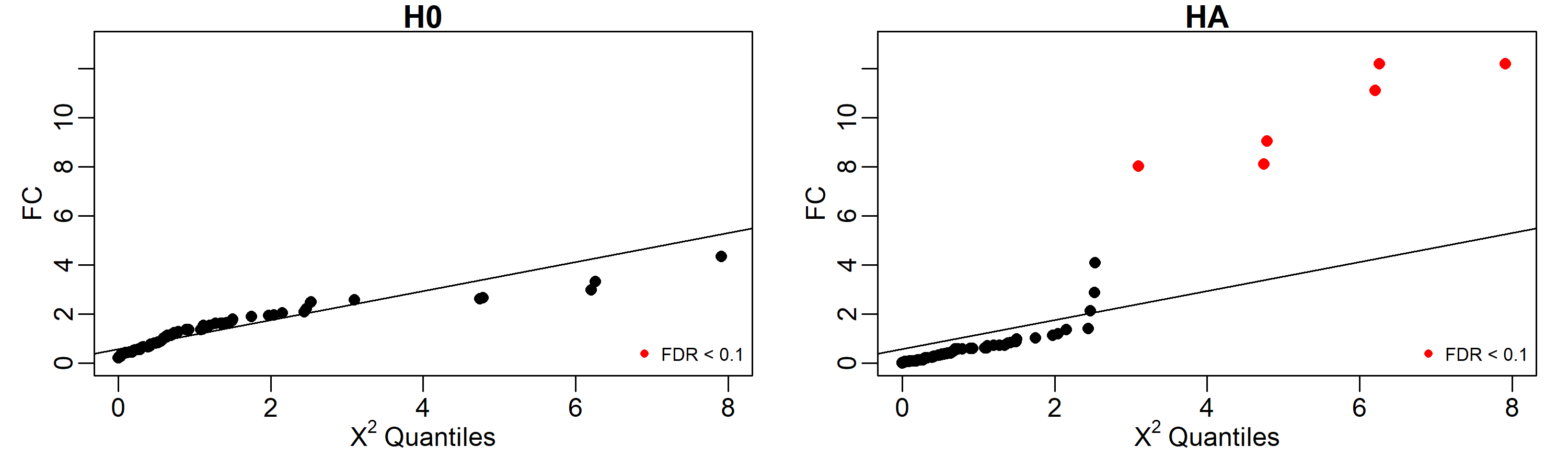
# y_ng59 1.138659e-15As is shown below, under the H0, none of the genes shown a significative difference in regulatory profiles using an FDR cut-off of 0.1, but under the HA, the 6 genes involved in the perturbation (50, 11, 2, 10, 5, and 3) are identified as perturbed.
head(outputH0$diffRegulation, n = 10)
#    gene     distance        Z       FC    p.value     p.adj
# 59 ng59 1.138659e-15 2.497859 4.338493 0.03725989 0.6411916
# 32 ng32 9.970451e-16 2.081719 3.326448 0.06817394 0.6411916
# 72 ng72 9.452170e-16 1.917581 2.989608 0.08380044 0.6411916
# 89 ng89 8.924023e-16 1.742758 2.664849 0.10258758 0.6411916
# 12 ng12 8.851226e-16 1.718018 2.621550 0.10542145 0.6411916
# 17 ng17 8.784453e-16 1.695183 2.582145 0.10807510 0.6411916
# 31 ng31 8.621191e-16 1.638760 2.487057 0.11478618 0.6411916
# 95 mt-5 8.578947e-16 1.624022 2.462743 0.11657501 0.6411916
# 57 ng57 8.141541e-16 1.467912 2.218015 0.13640837 0.6411916
# 77 ng77 7.888569e-16 1.374548 2.082321 0.14901342 0.6411916

head(outputHA$diffRegulation, n = 10)
#    gene   distance        Z        FC      p.value      p.adj
# 2   ng2 0.023526702 2.762449 12.193413 0.0004795855 0.02414332
# 50 ng50 0.023514429 2.761550 12.180695 0.0004828665 0.02414332
# 11 ng11 0.022443941 2.681598 11.096894 0.0008647241 0.02882414
# 3   ng3 0.020263415 2.508478  9.045415 0.0026335445 0.06583861
# 10 ng10 0.019194561 2.417929  8.116328 0.0043868326 0.07711821
# 5   ng5 0.019079975 2.407977  8.019712 0.0046270923 0.07711821
# 31 ng31 0.013632541 1.865506  4.094085 0.0430335257 0.61476465
# 96 mt-6 0.011401177 1.589757  2.863536 0.0906081350 0.90977795
# 59 ng59 0.009835354 1.368238  2.130999 0.1443466682 0.90977795
# 62 ng62 0.007995812 1.067193 1.408408 0.2353209153 0.90977795Results can be easily displayed using quantile-quantile plots. Here
we labeled in red the identified perturbed genes with FDR < 0.1.
par(mfrow=c(2,1), mar=c(3,3,1,1), mgp=c(1.5,0.5,0))
set.seed(1)
qChisq <- rchisq(100,1)
geneColor <- rev(ifelse(outputH0$diffRegulation$p.adj < 0.1, 10,1))
qqplot(qChisq, outputH0$diffRegulation$FC, pch = 16, main = 'H0', col = geneColor,
       xlab = expression(X^2~Quantiles), ylab = 'FC', xlim=c(0,8), ylim=c(0,13))
qqline(qChisq)
legend('bottomright', legend = c('FDR < 0.1'), pch = 16, col = 'red', bty='n', cex = 0.7)

geneColor <- rev(ifelse(outputHA$diffRegulation$p.adj < 0.1, 'red', 'black'))
qqplot(qChisq, outputHA$diffRegulation$FC, pch = 16, main = 'HA', col = geneColor,
       xlab = expression(X^2~Quantiles), ylab = 'FC', xlim=c(0,8), ylim=c(0,13))
qqline(qChisq)
legend('bottomright', legend = c('FDR < 0.1'), pch = 16, col = 'red', bty='n', cex = 0.7)To cite scTenifoldNet in publications use:
Daniel Osorio, Yan Zhong, Guanxun Li, Jianhua Huang and James Cai (2019). scTenifoldNet: Construct and Compare scGRN from Single-Cell Transcriptomic Data. R package version 1.2.0. https://CRAN.R-project.org/package=scTenifoldNet
A BibTeX entry for LaTeX users is
  @Manual{,
    title = {scTenifoldNet: Construct and Compare scGRN from Single-Cell Transcriptomic Data},
    author = {Daniel Osorio and Yan Zhong and Guanxun Li and Jianhua Huang and James Cai},
    year = {2019},
    note = {R package version 1.2.0},
    url = {https://CRAN.R-project.org/package=scTenifoldNet},
  }