The goal of rjqpd is to implement the Johnson
Quantile-Parameterised distribution system in R. It provides the density
function, cumulative distribution function, quantile function and random
sampling function in their usual form:
djqpd - calculates the density function (PDF)pjqpd - calculates the cumulative distribution function
(CDF)qjqpd - calculates the quantile function (QF)rjqpd - generates random samplesA common problem in data analysis is encountering continuous uncertainties that are not easily characterised by well known parametric, continuous probability distributions. Often the underlying process that generated the data is unknown or is inconvenient to express in closed form. In these cases one typically has to resort to curve fitting a distribution to a set of probability-quantile pairs without the guarantee that the best-fit distribution will pass through the assessed points exactly.
The Johnson Quantile-Parameterised Distribution (J-QPD) system is a novel approach to this problem first developed in a paper by Hadlock and Bickel (2017) in Decision Analysis Vol. 14, No. 1.
Their approach is to extend the Johnson Distribution System in a way such that the distributions constructed honour exactly a symmetric percentile triplet of quantile assessments (e.g. 15th, 50th, 85th) on a bounded or semi-bounded domain. By parameterising the distribution in this way the need for curve fitting can be eliminated.
The rjqpd package is not yet available on CRAN.
You can install the latest development version of rjqpd
using:
devtools::install_github("bobbyingram/rjqpd")The base function of the package is the jqpd class
constructor:
jqpd()This function takes the convenient symmetric percentile triplet quantile parameterisation and computes a set of constants required to calculate the distribution functions.
This is a basic example to show how to calculate the parameters of a bounded Johnson Quantile-Parameterised distribution from the quantiles of a symmetric percentile triplet (SPT).
library(rjqpd)

# alpha = 0.1 indicates a symmetric percentile triplet (SPT) of (0.1, 0.5, 0.9)
alpha <- 0.1
# we parameterise using some quantile values corresponding to the SPT above.
quantiles <- c(0.32, 0.40, 0.60)
params <- jqpd(quantiles, lower = 0, upper = 1, alpha = alpha)

# The CDF should return the (SPT) at the quantile values:
pjqpd(quantiles, params)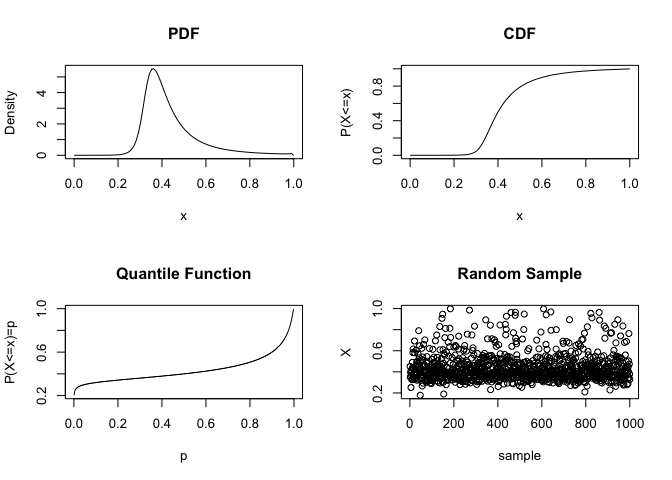
#> [1] 0.1 0.5 0.9The plot_jqpd function produces a simple summary plot
showing the density, cumulative distribution function, quantile function
and 1000 random samples:
plot_jqpd(params)
We also provide some basic summary statistics functions:
jqpd_mean - calculates the meanjqpd_var - calculates the variancejqpd_sd - calculates the standard deviationjqpd_skewness - calculates the skewnessjqpd_kurtosis - calculates the kurtosisjqpd_mean(params)
#> [1] 0.4350185jqpd_var(params)
#> [1] 0.01604665jqpd_sd(params)
#> [1] 0.1266754jqpd_skewness(params)
#> [1] 1.69221jqpd_kurtosis(params)
#> [1] 6.464129