

![]()
![]()
![]()
The rangr package is designed to simulate a species range dynamics. This new tool mimics the essential processes that shape population numbers and spatial distribution: local dynamics and dispersal. Simulations can be run in a spatially explicit and dynamic environment, facilitating population projections in response to climate or land-use changes. By using different sampling schemes and observational error distributions, the structure of the original survey data can be reproduced, or pure random sampling can be mimicked.
The study is supported by the National Science Centre, Poland, grant no. 2018/29/B/NZ8/00066 and the Poznań Supercomputing and Networking Centre (grant no. 403).
rangr is available from CRAN, so you can install it with:
install.packages("rangr")You can install the development version from R-universe or GitHub with:
install.packages("rangr", repos = "https://ropensci.r-universe.dev")
# or
devtools::install_github("ropensci/rangr")Here’s an example of how to use the rangr package.
Example maps available in rangr in the Cartesian coordinate system:
n1_small.tifn1_big.tifK_small.tifK_small_changing.tifK_big.tifExample maps available in rangr in the longitude/latitude coordinate system:
n1_small_lon_lat.tifn1_big_lon_lat.tifK_small_lon_lat.tifK_small_changing_lon_lat.tifK_big_lon_lat.tifYou can find additional information about these data sets in help files:
library(rangr)

?n1_small.tif
?K_small.tif
Two of the available datasets, n1_small.tif and
K_small.tif, represent the abundance of a virtual species
at the starting point of a simulation and the carrying capacity of the
environment, respectively. Both of these objects refer to the same
relatively small area, so they are ideal for demonstrating the usage of
the package. To view these maps and their dimensions, you can use the
following commands:
library(terra)
#> terra 1.7.55

n1_small <- rast(system.file("input_maps/n1_small.tif", package = "rangr"))
K_small <-  rast(system.file("input_maps/K_small.tif", package = "rangr"))
You can also use the plot function from the
terra package to visualize these maps:
plot(c(n1_small, K_small))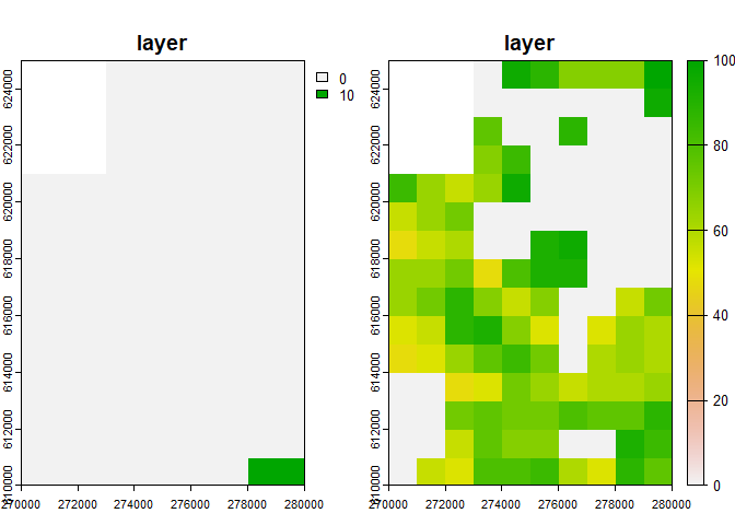
To create a sim_data object containing the necessary
information to run a simulation, use the initialise()
function. For example:
sim_data_01 <- initialise(
  n1_map = n1_small,
  K_map = K_small,
  r = log(2),
  rate = 1 / 1e3
)
Here, we set the intrinsic population growth rate to
log(2) and the rate parameter that is related to the kernel
function describing dispersal to 1/1e3.
To see the summary of the sim_data object:
summary(sim_data_01)
#> Summary of sim_data object
#>
#> n1 map summary:
#>    Min. 1st Qu.  Median    Mean 3rd Qu.    Max.    NA's
#>  0.0000  0.0000  0.0000  0.1449  0.0000 10.0000      12
#>
#> Carrying capacity map summary:
#>    Min. 1st Qu.  Median    Mean 3rd Qu.    Max.    NA's
#>    0.00    0.00   56.00   44.84   72.00  100.00      12
#>
#> growth        gompertz
#> r               0.6931
#> A                    -
#> kernel_fun        rexp
#> dens_dep           K2N
#> border       reprising
#> max_dist          4000
#> changing_env     FALSE
#> dlist TRUETo run a simulation, use the sim() function, which takes
a sim_data object and the specified number of time steps as
input parameters. For example:
sim_result_01 <- sim(obj = sim_data_01, time = 100)To see the summary of the sim_result_01 object:
summary(sim_result_01)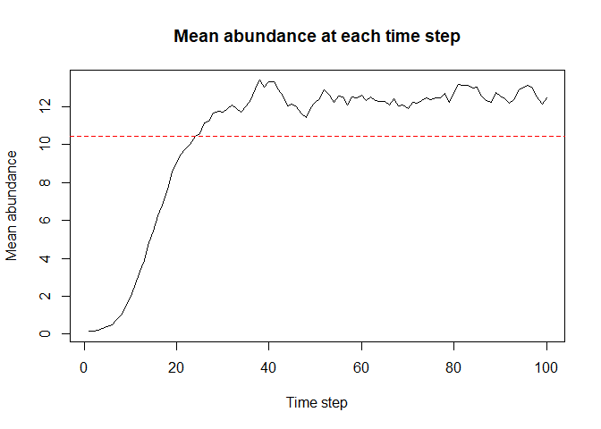
#> Summary of sim_results object
#>
#> Simulation summary:
#>
#> simulated time   100
#> extinction     FALSE
#>
#> Abundances summary:
#>    Min. 1st Qu.  Median    Mean 3rd Qu.    Max.    NA's
#>    0.00    0.00   12.00   10.45   19.00   54.00    1200
Note that this is a simple example and there are many more parameters
that can be set for initialise() and sim().
See the documentation for the rangr package for more
information.
You can use rangr to visualise selected time steps from
the simulation. The plot() method is used to generate the
plot. Here’s an example:
# generate visualisation
plot(sim_result_01,
  time_points = c(1, 10, 25, 50),
  template = sim_data_01$K_map
)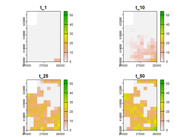
#> class       : SpatRaster
#> dimensions  : 15, 10, 4  (nrow, ncol, nlyr)
#> resolution  : 1000, 1000  (x, y)
#> extent      : 270000, 280000, 610000, 625000  (xmin, xmax, ymin, ymax)
#> coord. ref. : ETRS89 / Poland CS92
#> source(s)   : memory
#> names       : t_1, t_10, t_25, t_50
#> min values  :   0,    0,    0,    0
#> max values  :  10,   19,   27,   36
You can adjust the breaks parameter to get more breaks
on the colorscale:
# generate visualisation with more breaks
plot(sim_result_01,
  time_points = c(1, 10, 25, 50),
  breaks = seq(0, max(sim_result_01$N_map + 5, na.rm = TRUE), by = 5),
  template = sim_data_01$K_map
)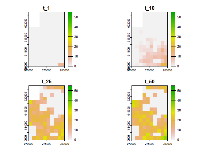
#> class       : SpatRaster
#> dimensions  : 15, 10, 4  (nrow, ncol, nlyr)
#> resolution  : 1000, 1000  (x, y)
#> extent      : 270000, 280000, 610000, 625000  (xmin, xmax, ymin, ymax)
#> coord. ref. : ETRS89 / Poland CS92
#> source(s)   : memory
#> names       : t_1, t_10, t_25, t_50
#> min values  :   0,    0,    0,    0
#> max values  :  10,   19,   27,   36
If you prefer working on raster you can also transform any
sim_result object into SpatRaster using
to_rast() function:
# raster construction
my_rast <- to_rast(
  sim_result_01,
  time_points = 1:sim_result_01$simulated_time,
  template = sim_data_01$K_map
)

# print raster
print(my_rast)
#> class       : SpatRaster
#> dimensions  : 15, 10, 100  (nrow, ncol, nlyr)
#> resolution  : 1000, 1000  (x, y)
#> extent      : 270000, 280000, 610000, 625000  (xmin, xmax, ymin, ymax)
#> coord. ref. : ETRS89 / Poland CS92
#> source(s)   : memory
#> names       : t_1, t_2, t_3, t_4, t_5, t_6, ...
#> min values  :   0,   0,   0,   0,   0,   0, ...
#> max values  :  10,  11,  14,  16,  20,  13, ...
And then visualise it using plot() function:
# plot selected time points
plot(my_rast, c(1, 10, 25, 50))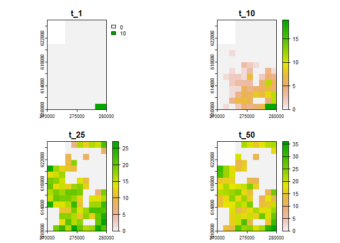
To cite rangr use citation() function:
library(rangr)
citation("rangr")Please note that this package is released with a Contributor Code of Conduct. By contributing to this project, you agree to abide by its terms.