Overview To start using the installed package:
library(radsafer)The radsafer package was developed with these goals:
Provide functions that are commonly used in radiation safety
Provide easy access to data provided in the RadData package
Share some less commonly-used functions that may be of significant value to workers in instrumentation and modeling
Related functions are identified as members of these families:
decay corrections
radionuclides
rad measurements
mcnp tools
A few functions stand alone.
This framework makes it a little easier to find the function you want - the help file for each function lists related functions.
Radsafer includes several functions to manage radioactive decay corrections:
dk_correct provides decay corrected activity or activity-dependent value, such as instrument response rate or dose rate. The computation is made either based on a single radionuclide, or based on user-provided half-life, with time unit. The differential time is either computed based on dates entered or time lapsed based on the time unit.
Obtain a correction factor for a source to be used today based on a
calibration on date1. Allow date2 to be the
default system date.
dk_correct(half_life = 10,
           time_unit = "y",
           date1 = "2010-01-01")
#>  half_life RefValue    RefDate   TargDate  dk_value
#>         10        1 2010-01-01 2023-07-11 0.3916907
Use this function to correct for the value needed on dates it was
used. Let the function obtain the half-life from the ICRP Publication
107 decay data in the RadData R package. In the example, we
have a disk source with an original count rate of 10000 cpm:
dk_correct(RN_select = "Sr-90",
           date1 = "2005-01-01",
           date2 = c("2009-01-01","2009-10-01"),
           A1 = 10000)
#>     RN half_life units decay_mode
#>  Sr-90     28.79     y         B-
#>
#>     RN RefValue    RefDate   TargDate dk_value
#>  Sr-90    10000 2005-01-01 2009-01-01 9081.895
#>  Sr-90    10000 2005-01-01 2009-10-01 8919.954
Reverse decay - find out what readings should have been in the past given today’s reading of 3000
dk_correct(RN_select = "Cs-137",
  date1 = "2019-01-01",
  date2 = c("2009-01-01","1999-01-01"),
  A1 = 3000)
#>      RN half_life units decay_mode
#>  Cs-137   30.1671     y         B-
#>
#>      RN RefValue    RefDate   TargDate dk_value
#>  Cs-137     3000 2019-01-01 2009-01-01 3774.795
#>  Cs-137     3000 2019-01-01 1999-01-01 4749.991
Other decay functions answer the following questions:
How long does it take to decay something with a given activity, or how old is a sample if it has decayed from? dk_time
Given a percentage reduction in activity, how many half-lives have passed.dk_pct_to_num_half_life
Given two or more data points, estimate the half-life: half_life_2pt
Search by alpha, beta, photon or use the general screen option.
RN_search_phot_by_E allows screening based on energy,
half-life, and minimum probability. Also available are
RN_search_alpha_by_E, RN_search_beta_by_E, and
bin_screen_phot. RN_bin_screen_phot allows
limiting searches to radionuclides with emissions in an energy bin of
interest with additional filters for not having photons in other
specified energy bins. Results for all these search functions may be
plotted with RN_plot_spectrum.
Here’s a search for photon energy between 0.99 and 1.01 MeV, half-life between 13 and 15 minutes, and probability at least 1e-3
search_results <- RN_search_phot_by_E(0.99, 1.01, 13 * 60, 15 * 60, 1e-3)| RN | code_AN | E_MeV | prob | half_life | units | decay_constant |
|---|---|---|---|---|---|---|
| Pr-136 | G | 0.99100 | 0.0016768 | 13.10 | m | 0.0008819 |
| Pr-136 | G | 1.00070 | 0.0503040 | 13.10 | m | 0.0008819 |
| Re-178 | G | 1.00440 | 0.0057600 | 13.20 | m | 0.0008752 |
| Pr-147 | G | 0.99597 | 0.0083220 | 13.40 | m | 0.0008621 |
| Nb-88 | G | 0.99760 | 0.0041000 | 14.50 | m | 0.0007967 |
| Mo-101 | G | 1.00740 | 0.0017300 | 14.61 | m | 0.0007907 |
| Sm-140 | G | 0.99990 | 0.0012000 | 14.82 | m | 0.0007795 |
RN_plot_spectrum(search_results)
#> [1] "No matches"
You can also plot a spectrum in one step, skipping the data save:
 RN_plot_spectrum(
   desired_RN = c("Pu-238", "Pu-239", "Am-241"), rad_type = "A",
   photon = FALSE, prob_cut = 0.01, log_plot = 0)
The RN_index_screen function helps find a radionuclide
of interest based on decay mode, half-life, and total emission
energy.
In this example, we search for radionuclides decaying by spontaneous fission with half-lives between 6 months and 2 years.
RNs_selected <- RN_index_screen(dk_mode = "SF", min_half_life_seconds = 0.5 * 3.153e7, max_half_life_seconds = 2 * 3.153e7)| RN | half_life | units |
|---|---|---|
| Es-254 | 275.7 | d |
| Cf-248 | 334.0 | d |
Other radionuclides family functions:
Obtain a specific activity with RN_Spec_Act.
Find a potential radionuclide parent with RN_find_parent.
RN_find_parent("Th-230")
#>       RN
#> 1 Ac-230
#> 2 Pa-230
#> 3 U-234air_dens_cf Correct vented ion chamber readings based on difference in air pressure (readings in degrees Celsius and mm Hg):
air_dens_cf(T.actual = 30, P.actual = 760, T.ref = 20, P.ref = 760)
#> [1] 1.034112
Let’s try it out combined with the instrument reading:
rdg <- 100
(rdg_corrected <- rdg * air_dens_cf(T.actual = 30, P.actual = 760, T.ref = 20, P.ref = 760))
#> [1] 103.4112
neutron_geom_cf
Correct for geometry when reading a close neutron source. Example: neutron rem detector with a radius of 11 cm and source near surface:
neutron_geom_cf(11.1, 11)
#> [1] 0.7236467
disk_to_disk_solid_angle
Correct for a mismatch between the source calibration of a counting system and the item being measured. A significant factor in the counting efficiency is the solid angle from the source to the detector. You can also check for the impact of an item not being centered with the detector.
Example: You are counting an air sample with an active collection diameter of 45 mm, your detector has a radius of 25 mm and there is a gap between the two of 5 mm. (The function is based on radius, not diameter so be sure to divide the diameter by two.) The relative solid angle is:
(as_rel_solid_angle <- as.numeric(disk_to_disk_solid_angle(r.source = 45/2, gap = 20, r.detector = 12.5, runs = 1e4, plot.opt = "n")))
#> [1] 0.047469927 0.002120278
An optional plot is available in 2D or 3D:
  library(ggplot2)
theme_update(# axis labels
             axis.title = element_text(size = 7),
             # tick labels
             axis.text = element_text(size = 5),
             # title
             title = element_text(size = 5))
(as_rel_solid_angle <- as.numeric(disk_to_disk_solid_angle(r.source = 45/2, gap = 20, r.detector = 12.5, runs = 1e4, plot.opt = "3d")))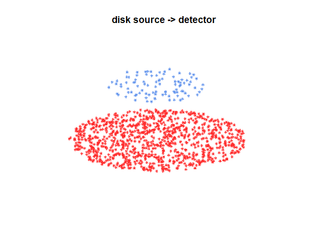
#> [1] 0.047585442 0.002137657Continuing the example: the only calibration source you had available with the appropriate isotope has an active diameter of 20 mm. Is this a big deal? Let’s estimate the relative solid angle of the calibration, then take a ratio of the two.
(cal_rel_solid_angle <- disk_to_disk_solid_angle(r.source = 20, gap = 20, r.detector = 12.5, runs = 1e4, plot.opt = "n"))
#>   mean_eff         SEM
#>  0.0528169 0.002243531
Correct for the mismatch:
(cf <- cal_rel_solid_angle / as_rel_solid_angle)
#>  mean_eff      SEM
#>  1.109938 1.049528
This makes sense - the air sample has particles originating outside the source radius, so more of them will be lost, thus an adjustment is needed for the activity measurement.
scaler_sim
Scaler counts: obtain quick distributions for parameters of interest:
scaler_sim(true_bkg = 50, true_samp = 10, ct_time = 20, trials = 1e5)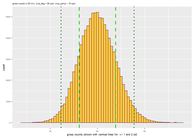
rate_meter_sim
Rate meters: In the ratemeter simulation, readings are plotted once per second for a default time of 600 seconds. The meter starts with a reading of zero and builds up based on the time constant. Resolution uncertainty is established to express the uncertainty from reading an analog scale, including the instability of its readings. Many standard references identify the precision or resolution uncertainty of analog readings as half of the smallest increment. This should be considered the single coverage uncertainty for a very stable reading. When a reading is not very stable, evaluation of the reading fluctuation is evaluated in terms of numbers of scale increments covered by meter indication over a reasonable evaluation period. Example with default time constant:
rate_meter_sim(cpm_equilibrium = 270, meter_scale_increments = seq(100, 1000, 20))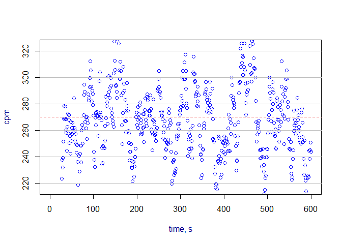
To estimate time constant, use tau.estimate
Given a dose rate, dose allowed, and a safety margin (default = 20%),
calculate stay time with: stay_time
stay_time(dose_rate = 120, dose_allowed = 100, margin =  20)
#> [1] "Time allowed is 40 minutes"
#> [1] 40Given a set of radiation levels through varying thicknesses of material, compute the half-values, tenth-values, and homogeneity coefficients.
hvl(x = mm_Al, y = mR_h)
#>   thickness response        mu      hvl      tvl        hc
#> 1         0    7.428        NA       NA       NA        NA
#> 2         1    6.272 0.1691614 4.097550 13.61177 0.9676121
#> 3         2    5.325 0.1636826 4.234704 14.06738 0.9810918
#> 4         3    4.535 0.1605876 4.316317 14.33850 0.9745802
#> 5         4    3.878 0.1565055 4.428899 14.71248 0.9984235
#> 6 5 3.317 0.1562588 4.435892 14.73571 NAIf you create MCNP inputs, these functions may be helpful:
mcnp_sdef_erg_line Obtain emission data from the
RadData package for use with the radiation transport code,
MCNP, when you want a “line” source from individual radionuclides. Use
mcnp_sdef_erg_hist when you have histogram data and
want to format it nicely for MCNP.
mcnp_matrix_rotations
mcnp_matrix_rotations("z", 90)
#> [1]  0  1  0 -1  0  0  0  0  1
mcnp_cone_angle This is just the square of the tangent of the angle in radians, but the argument used here is degree.
mcnp_cone_angle(30)
#> [1] 0.3333333
mcnp_mesh_bins This helps identify the x, y, or z parameter of a simple geometric mesh tally. Select a center of interest, the width of this center mesh, then minimum and maximum limits on the extent of the entire mesh. Repeat for the other dimensions.
mcnp_mesh_bins(target = 30, width = 10, lowest_less = 0, highest_less = 15, highest_high = 304.8, lowest_high = 250)
#> low_set high_set width numblocks
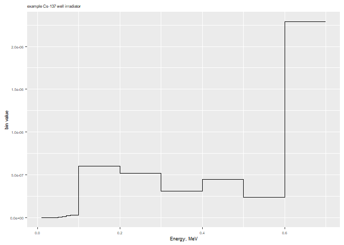
#> 5 295 10 29mcnp_plot_out_spec
For MCNP outputs, plot the results of a tally with
energy bins. The fastest way to do this is with
mcnp_scan2plot.
Alternatively, if you want to get your data into R, first save it in
a text file and import it to R. (Base R provides methods with
read.table or you might prefer options from the
readr or readxl packages.) Or you can copy and
paste your data using mcnp_scan_save. You can then plot
with mcnp_plot_out_spec (below) or design your own
plot.
mcnp_plot_out_spec(photons_cs137_hist, 'example Cs-137 well irradiator')