![]()
![]()
The goal of quickr is to make your R code run quicker.
R is an extremely flexible and dynamic language, but that flexibility and dynamicism can come at the expense of speed. This package lets you trade back some of that flexibility for some speed, for the context of a single function.
The main exported function is quick(). Here is how you
use it:
library(quickr)

convolve <- quick(function(a, b) {
  declare(type(a = double(NA)),
          type(b = double(NA)))
  ab <- double(length(a) + length(b) - 1)
  for (i in seq_along(a)) {
    for (j in seq_along(b)) {
      ab[i+j-1] <- ab[i+j-1] + a[i] * b[j]
    }
  }
  ab
})
quick() returns a quicker R function. How much quicker?
Let’s benchmark it! For reference, we’ll also compare it to a pure-C
implementation.
slow_convolve <- function(a, b) {
  declare(type(a = double(NA)),
          type(b = double(NA)))
  ab <- double(length(a) + length(b) - 1)
  for (i in seq_along(a)) {
    for (j in seq_along(b)) {
      ab[i+j-1] <- ab[i+j-1] + a[i] * b[j]
    }
  }
  ab
}

library(quickr)
quick_convolve <- quick(slow_convolve)

convolve_c <- inline::cfunction(
  sig = c(a = "SEXP", b = "SEXP"), body = r"({
    int na, nb, nab;
    double *xa, *xb, *xab;
    SEXP ab;

    a = PROTECT(Rf_coerceVector(a, REALSXP));
    b = PROTECT(Rf_coerceVector(b, REALSXP));
    na = Rf_length(a); nb = Rf_length(b); nab = na + nb - 1;
    ab = PROTECT(Rf_allocVector(REALSXP, nab));
    xa = REAL(a); xb = REAL(b); xab = REAL(ab);
    for(int i = 0; i < nab; i++) xab[i] = 0.0;
    for(int i = 0; i < na; i++)
        for(int j = 0; j < nb; j++)
            xab[i + j] += xa[i] * xb[j];
    UNPROTECT(3);
    return ab;
})")


a <- runif(100000); b <- runif(100)

timings <- bench::mark(
  r = slow_convolve(a, b),
  quickr = quick_convolve(a, b),
  c = convolve_c(a, b),
  min_time = 2
)
timings
#> # A tibble: 3 × 6
#>   expression      min   median `itr/sec` mem_alloc `gc/sec`
#>   <bch:expr> <bch:tm> <bch:tm>     <dbl> <bch:byt>    <dbl>
#> 1 r             1.43s    1.43s     0.702     782KB    0.702
#> 2 quickr       2.63ms    2.7ms   355.        782KB    6.77
#> 3 c            4.92ms   5.22ms   189.        782KB    3.61
plot(timings) + bench::scale_x_bench_time(base = NULL)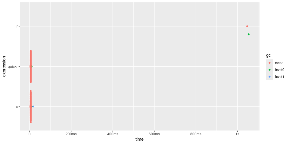
In the case of convolve(), quick() returns
a function approximately 200 times quicker, with performance
similar to the C function.
quick() can accelerate any R function, with some
restrictions:
declare().integer, double, logical, and
complex.NA values are not supported.#> [1] - : ! != (
#> [6] [ [<- [<<- { *
#> [11] / & && %*% %/%
#> [16] %% %o% ^ + <
#> [21] <- <<- <= = ==
#> [26] > >= | || $
#> [31] Arg Conj Fortran Im Mod
#> [36] Re abs acos all any
#> [41] array as.double as.integer asin atan
#> [46] backsolve break c cat cbind
#> [51] ceiling character chol chol2inv cos
#> [56] crossprod declare diag dim double
#> [61] drop exp floor for forwardsolve
#> [66] if ifelse integer is.null length
#> [71] log log10 logical matrix max
#> [76] min ncol next nrow numeric
#> [81] outer print prod qr.solve raw
#> [86] rbind rep.int repeat rev runif
#> [91] seq seq_along seq_len sin solve
#> [96] sqrt stop sum svd t
#> [101] tan tanh tcrossprod trunc which.max
#> [106] which.min whileMany of these restrictions are expected to be relaxed as the project matures. However, quickr is intended primarily for high-performance numerical computing, so features like polymorphic dispatch or support for complex or dynamic types are out of scope.
declare(type()) syntax:The shape and mode of all function arguments must be declared. Local and return variables may optionally also be declared.
declare(type()) also has support for declaring size
constraints, or size relationships between variables. Here are some
examples of declare calls:
declare(type(x = double(NA))) # x is a 1-d double vector of any length
declare(type(x = double(10))) # x is a 1-d double vector of length 10
declare(type(x = double(1)))  # x is a scalar double

declare(type(x = integer(2, 3)))  # x is a 2-d integer matrix with dim (2, 3)
declare(type(x = integer(NA, 3))) # x is a 2-d integer matrix with dim (<any>, 3)

# x is a 4-d logical matrix with dim (<any>, 24, 24, 3)
declare(type(x = logical(NA, 24, 24, 3)))

# x and y are 1-d double vectors of any length
declare(type(x = double(NA)),
        type(y = double(NA)))

# x and y are 1-d double vectors of the same length
declare(
  type(x = double(n)),
  type(y = double(n)),
)

# x and y are 1-d double vectors, where length(y) == length(x) + 2
declare(type(x = double(n)),
        type(y = double(n+2)))
Tip: declare shapes as specifically as you can. quickr uses these
size constraints both for compile-time checking and for choosing more
efficient implementations. For example, if you know a matrix is square,
declare it as type(A = double(n, n)) (not
double(n, k)). That can allow quickr to use a faster code
path for operations like solve(A, b). If the compiler can’t
prove a matrix is square, it may need to fall back to a more general
rectangular solver.
viterbiThe Viterbi algorithm is an example of a dynamic programming
algorithm within the family of Hidden Markov Models (https://en.wikipedia.org/wiki/Viterbi_algorithm). Here,
quick() makes viterbi() approximately 50 times
faster.
slow_viterbi <- function(observations, states, initial_probs, transition_probs, emission_probs) {
    declare(
      type(observations = integer(num_steps)),
      type(states = integer(num_states)),
      type(initial_probs = double(num_states)),
      type(transition_probs = double(num_states, num_states)),
      type(emission_probs = double(num_states, num_obs)),
    )

    trellis <- matrix(0, nrow = length(states), ncol = length(observations))
    backpointer <- matrix(0L, nrow = length(states), ncol = length(observations))
    trellis[, 1] <- initial_probs * emission_probs[, observations[1]]

    for (step in 2:length(observations)) {
      for (current_state in 1:length(states)) {
        probabilities <- trellis[, step - 1] * transition_probs[, current_state]
        trellis[current_state, step] <- max(probabilities) * emission_probs[current_state, observations[step]]
        backpointer[current_state, step] <- which.max(probabilities)
      }
    }

    path <- integer(length(observations))
    path[length(observations)] <- which.max(trellis[, length(observations)])
    for (step in seq(length(observations) - 1, 1)) {
      path[step] <- backpointer[path[step + 1], step + 1]
    }

    out <- states[path]
    out
}

quick_viterbi <- quick(slow_viterbi)

set.seed(1234)
num_steps <- 16
num_states <- 8
num_obs <- 16

observations <- sample(1:num_obs, num_steps, replace = TRUE)
states <- 1:num_states
initial_probs <- runif (num_states)
initial_probs <- initial_probs / sum(initial_probs)  # normalize to sum to 1
transition_probs <- matrix(runif (num_states * num_states), nrow = num_states)
transition_probs <- transition_probs / rowSums(transition_probs)  # normalize rows
emission_probs <- matrix(runif (num_states * num_obs), nrow = num_states)
emission_probs <- emission_probs / rowSums(emission_probs)  # normalize rows

timings <- bench::mark(
  slow_viterbi = slow_viterbi(observations, states, initial_probs,
                              transition_probs, emission_probs),
  quick_viterbi = quick_viterbi(observations, states, initial_probs,
                                transition_probs, emission_probs)
)
timings
#> # A tibble: 2 × 6
#>   expression         min   median `itr/sec` mem_alloc `gc/sec`
#>   <bch:expr>    <bch:tm> <bch:tm>     <dbl> <bch:byt>    <dbl>
#> 1 slow_viterbi  170.18µs 186.23µs     5011.    1.59KB     12.4
#> 2 quick_viterbi   2.44µs   2.72µs   349107.        0B      0
plot(timings)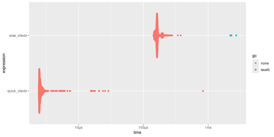
Simulate how heat spreads over time across a 2D grid, using the finite difference method applied to the Heat Equation.
Note the use of local closures within the quick function. Here,
quick() returns a function approximately 20 times faster.
The speedup is relatively modest because the core operation of computing
the laplacian is already expressed as a vectorized operation. If we were
instead comparing against for loops that operate on
individual array elements, the speedup would be much more substantial.
In general, idiomatic vectorized R code is quite fast already!
diffuse_heat <- function(nx, ny, dx, dy, dt, k, steps) {
  declare(
    type(nx = integer(1)),
    type(ny = integer(1)),
    type(dx = integer(1)),
    type(dy = integer(1)),
    type(dt = double(1)),
    type(k = double(1)),
    type(steps = integer(1))
  )

  temp <- matrix(0, nx, ny)
  temp[nx %/% 2L, ny %/% 2L] <- 100

  apply_boundary_conditions <- function(temp) {
    temp[1, ] <- 0
    temp[nx, ] <- 0
    temp[, 1] <- 0
    temp[, ny] <- 0
    temp
  }

  update_temperature <- function(temp) {
    temp_new <- temp

    i <- 2:(nx - 1)
    j <- 2:(ny - 1)

    laplacian <-
      (temp[i + 1, j] - 2 * temp[i, j] + temp[i - 1, j]) / dx ^ 2 +
      (temp[i, j + 1] - 2 * temp[i, j] + temp[i, j - 1]) / dy ^ 2

    temp_new[i, j] <- temp[i, j] + k * dt * laplacian
    temp_new
  }

  for (step in seq_len(steps)) {
    temp <- temp |>
      apply_boundary_conditions() |>
      update_temperature()
  }

  temp
}


quick_diffuse_heat <- quick(diffuse_heat)

# Parameters
nx <- 100L      # Grid size in x
ny <- 100L      # Grid size in y
dx <- 1L        # Grid spacing
dy <- 1L        # Grid spacing
dt <- 0.01      # Time step
k <- 0.1        # Thermal diffusivity
steps <- 500L   # Number of time steps

timings <- bench::mark(
  diffuse_heat = diffuse_heat(nx, ny, dx, dy, dt, k, steps),
  quick_diffuse_heat = quick_diffuse_heat(nx, ny, dx, dy, dt, k, steps)
)
#> Warning: Some expressions had a GC in every iteration; so filtering is
#> disabled.
summary(timings, relative = TRUE)
#> Warning: Some expressions had a GC in every iteration; so filtering is
#> disabled.
#> # A tibble: 2 × 6
#>   expression           min median `itr/sec` mem_alloc `gc/sec`
#>   <bch:expr>         <dbl>  <dbl>     <dbl>     <dbl>    <dbl>
#> 1 diffuse_heat        13.6   16.8       1       4893.      Inf
#> 2 quick_diffuse_heat   1      1        16.7        1       NaN
plot(timings)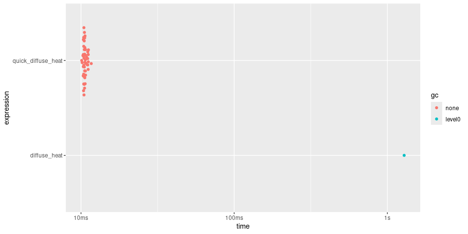
Here is quickr used to calculate a rolling mean. The CRAN package RcppRoll already provides a highly optimized rolling mean, which we include in the benchmarks for comparison.
slow_roll_mean <- function(x, weights, normalize = TRUE) {
  declare(
    type(x = double(NA)),
    type(weights = double(NA)),
    type(normalize = logical(1))
  )
  out <- double(length(x) - length(weights) + 1)
  n <- length(weights)
  if (normalize)
    weights <- weights/sum(weights)*length(weights)

  for(i in seq_along(out)) {
    out[i] <- sum(x[i:(i+n-1)] * weights) / length(weights)
  }
  out
}

quick_roll_mean <- quick(slow_roll_mean)

x <- dnorm(seq(-3, 3, len = 100000))
weights <- dnorm(seq(-1, 1, len = 100))

timings <- bench::mark(
  r = slow_roll_mean(x, weights),
  rcpp = RcppRoll::roll_mean(x, weights = weights),
  quickr = quick_roll_mean(x, weights = weights)
)
#> Warning: Some expressions had a GC in every iteration; so filtering is
#> disabled.
timings
#> # A tibble: 3 × 6
#>   expression      min   median `itr/sec` mem_alloc `gc/sec`
#>   <bch:expr> <bch:tm> <bch:tm>     <dbl> <bch:byt>    <dbl>
#> 1 r           187.9ms  292.3ms      3.42  124.24MB    10.3
#> 2 rcpp        20.12ms   20.4ms     48.9     4.46MB     0
#> 3 quickr       6.82ms    7.2ms    133.    781.35KB     1.99

timings$expression <- factor(names(timings$expression), rev(names(timings$expression)))
plot(timings) + bench::scale_x_bench_time(base = NULL)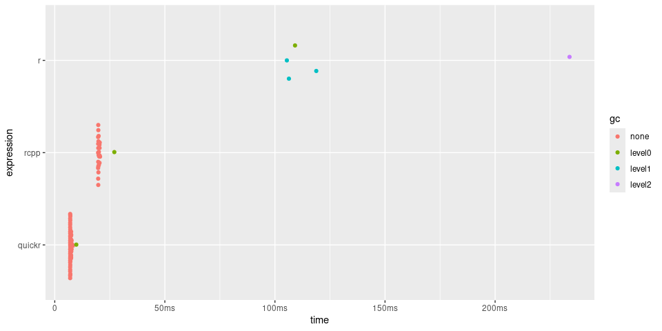
fastLm)quickr supports a variety of matrix operations from base R, including
most of the common linear algebra functions like %*%,
crossprod(), tcrossprod(),
solve(), and chol(). Performance is generally
similar to running the same code in R itself, but as you start to chain
multiple operations in a function, you may see speed-ups due to reduced
interpreter overhead. Actual performance depends on the BLAS/LAPACK
libraries linked to your R build (e.g. OpenBLAS, MKL, Accelerate).
To illustrate, here is a benchmark showing a
fastLm-style implementation comparing base R, quickr, and
(for reference) a compiled RcppArmadillo implementation. The
fastLm function is adapted from the README of the
RcppArmadillo project.
# reference implementation
fast_lm_ref <- function(X, y) {
  fit <- lm(y ~ X - 1)
  s <- summary(fit)

  list(
    coefficients = unname(coef(fit)),
    stderr = unname(s$coefficients[, "Std. Error"]),
    df.residual = fit$df.residual
  )
}

# RcppArmadillo implementation
Rcpp::sourceCpp(
code = '
#include <RcppArmadillo/Lighter>
// [[Rcpp::depends(RcppArmadillo)]]

// [[Rcpp::export]]
Rcpp::List fast_lm_rcpp_armadillo(const arma::mat& X, const arma::colvec& y) {
    int n = X.n_rows, k = X.n_cols;

    arma::colvec coef = arma::solve(X, y);     // fit model y ~ X
    arma::colvec res  = y - X*coef;            // residuals
    double s2 = arma::dot(res, res) / (n - k); // std.errors of coefficients
    arma::colvec std_err = arma::sqrt(s2 * arma::diagvec(arma::pinv(arma::trans(X)*X)));

    return Rcpp::List::create(Rcpp::Named("coefficients") = coef,
                              Rcpp::Named("stderr")       = std_err,
                              Rcpp::Named("df.residual")  = n - k);
}')

# Plain R fast-path
fast_lm_r <- function(X, y) {
  declare(
    type(X = double(n, k)),
    type(y = double(n))
  )

  # analogous to arma::pinv()
  pinv_svd <- function(A, tol = NULL) {
    s <- svd(A)
    if (is.null(tol)) {
      tol <- max(dim(A)) * max(s$d) * .Machine$double.eps
    }
    d_inv <- ifelse(s$d > tol, 1 / s$d, 0)
    s$v %*% (d_inv * t(s$u))
  }

  df_residual <- nrow(X) - ncol(X)

  coef <- qr.solve(X, y) # analogous to arma::solve(X, y)
  res <- y - X %*% coef
  s2 <- drop(crossprod(res)) / df_residual

  XtX <- crossprod(X)
  XtX_pinv <- pinv_svd(XtX) # analogous to arma::pinv()
  std_err <- sqrt(s2 * diag(XtX_pinv))

  list(
    coefficients = coef,
    stderr = std_err,
    df.residual = df_residual
  )
}

# quickr func
quick_fast_lm <- quick(fast_lm_r)set.seed(1)
beta <- c(0.5, 1.0, -2.0, 10, 5)
X <- cbind(1, matrix(rnorm(3 * 10^5), ncol = 4))
y <- as.vector(X %*% beta + rnorm(nrow(X), sd = 2))
timings <- bench::mark(
`reference` = fast_lm_ref(X, y),
`RcppArmadillo` = fast_lm_rcpp_armadillo(X, y),
`plain R` = fast_lm_r(X, y),
`quickr` = quick_fast_lm(X, y)
)
timings
#> # A tibble: 4 × 6
#> expression min median `itr/sec` mem_alloc `gc/sec`
#> <bch:expr> <bch:tm> <bch:tm> <dbl> <bch:byt> <dbl>
#> 1 reference 65.18ms 65.41ms 13.9 29.6MB 13.9
#> 2 RcppArmadillo 5.56ms 7.86ms 110. 0B 0
#> 3 plain R 5.1ms 8.82ms 66.7 13.2MB 16.0
#> 4 quickr 2.22ms 2.66ms 256. 0B 0
plot(timings) + ggplot2::scale_y_discrete(limits = rev(c(
"reference", "RcppArmadillo", "plain R", "quickr"
)))
Use declare(parallel()) to annotate the next
for loop or sapply() call for OpenMP
parallelization. Parallel loops must be order-independent: avoid
shared-state updates or inter-iteration dependencies. OpenMP adds
overhead, so it can be slower for small workloads, but substantially
faster for larger ones.
Here is a concrete example using colSums(). At smaller
sizes, the quickr serial version is fastest (even faster than base
colSums()). As sizes grow, the two serial versions
converge, and the parallel version pulls ahead. However, the speedup is
not linear with core count (e.g., with 12 cores, the speedup is closer
to ~6x).
colSums_quick_parallel <- quick(function(x) {
  declare(type(x = double(NA, NA)))
  declare(parallel())
  sapply(seq_len(nrow(x)), \(r) sum(x[, r]))
})

colSums_quick <- quick(function(x) {
  declare(type(x = double(NA, NA)))
  sapply(seq_len(nrow(x)), \(r) sum(x[, r]))
})

r <- bench::press(
  n = 2^(4:14),
  {
    m <- array(runif(n * n), c(n, n))
    bench::mark(
      parallel = colSums_quick_parallel(m),
      quick = colSums_quick(m),
      base = colSums(m),
    )
  },
  .quiet = TRUE
)

library(ggplot2)
library(dplyr, warn.conflicts = FALSE)

r |>
  mutate(.before = 1,
         desc = attr(expression, "description")) |>
  select(desc, n, median) |>
  ggplot(aes(x = n, y = median, color = desc)) +
  geom_point() + geom_line() +
  scale_x_log10() + bench::scale_y_bench_time()
quickr does not set OpenMP thread counts. To control threads, set
OMP_NUM_THREADS (and optionally
OMP_THREAD_LIMIT or OMP_DYNAMIC) before
calling a compiled function, e.g.
Sys.setenv(OMP_NUM_THREADS = "4").
quickr in an R
packageWhen called in a package, quick() will pre-compile the
quick functions and place them in the ./src directory. Run
devtools::load_all() or
quickr::compile_package() to ensure that the generated
files in ./src and ./R are in sync with each
other.
In a package, you must provide a function name to
quick(). For example:
my_fun <- quick(name = "my_fun", function(x) ....)You can install quickr from CRAN with:
install.packages("quickr")You can install the development version of quickr from GitHub with:
# install.packages("pak")
pak::pak("t-kalinowski/quickr")
You will also need a C and Fortran compiler, preferably the same ones used to build R itself.
On macOS:
Make sure xcode tools and gfortran are installed, as described in https://mac.r-project.org/tools/. In Terminal, run:
sudo xcode-select --install
# curl -LO https://mac.r-project.org/tools/gfortran-12.2-universal.pkg # R 4.4
# sudo installer -pkg gfortran-12.2-universal.pkg -target /
curl -LO https://mac.r-project.org/tools/gfortran-14.2-universal.pkg   # R 4.5
sudo installer -pkg gfortran-14.2-universal.pkg -target /
Optional: install flang-new via Homebrew (used by
quickr on macOS when available):
brew install flangOn Windows:
On Linux: