In many pharmaceutical and biomedical applications such as assay validation, assessment of historical control data or the detection of anti-drug antibodies, prediction intervals are of use. The package predint provides functions to calculate bootstrap calibrated prediction intervals (or limits) for one or more future observations based on overdispersed binomial data, overdispersed Poisson data, as well as data that is modeled by linear random effects models fitted with lme4::lmer(). The main functions are:
beta_bin_pi() for beta-binomial observations
(overdispersion differs between clusters)
quasi_bin_pi() for quasi-binomial observations
(constant overdispersion between clusters)
neg_bin_pi() for negative_binomial observations
(overdispersion differs between clusters)
quasi_pois_pi() for quasi-Poisson observations
(constant overdispersion between clusters)
lmer_pi_futmat() for data that is modeled by a
linear random effects model. This function takes the experimental design
of the future observations into account if computed for \(M>1\) observations.
For all of these functions, it is assumed that the historical, as well as the future (or current) observations descend from the same data generating process.
You can install the released version of predint from CRAN with:
install.packages("predint")And the development version from GitHub with:
# install.packages("devtools")
devtools::install_github("MaxMenssen/predint")The following example is based on the scenario described in Menssen and Schaarschmidt 2019: Based on historical control data for the mortality of male B6C3F1-mice obtained in long term studies at the National Toxicology Program (NTP 2017), prediction intervals (PI) can be computed in order to validate the observed mortality in one concurrent (or future) control group.
Similarly to Menssen and Schaarschmidt 2019, it is assumed, that the
data is overdispersed binomial. Hence, the quasi_bin_pi()
function will be used in the following two examples.
In this example, the validation of one control group the is comprised
of 30 mice is of interest. For this purpose, a pointwise 95 % prediction
interval for one future observation is computed based on the historical
data. Since the underlying distribution is skewed, the lower and the
upper prediction limit are calibrated independently from each other (by
setting algorithm="MS22mod").
# load predint
library(predint)
#> Loading required package: ggplot2
#> Loading required package: lme4
#> Loading required package: Matrix
#> Loading required package: MASS
#>
#> Attaching package: 'predint'
#> The following object is masked from 'package:stats':
#>
#>     rnbinom

# Data set
# see Table 1 of the supplementary material of Menssen and Schaarschmidt 2019
mortality_HCD
#>    dead alive
#> 1    15    35
#> 2    10    40
#> 3    12    38
#> 4    12    38
#> 5    13    37
#> 6    11    39
#> 7    19    31
#> 8    11    39
#> 9    14    36
#> 10   21    29

# PI for one future control group comprised of 30 mice
pi_m1 <- quasi_bin_pi(histdat=mortality_HCD,
                      newsize=30,
                      traceplot = FALSE,
                      alpha=0.05,
                      algorithm="MS22mod")

pi_m1
#> Pointwise 95 % prediction interval for one future observation
#>
#>      lower    upper newsize
#> 1 2.176397 15.05858      30
The mortality of a concurrent control group is in line with the historical knowledge, if it is not lower than 2.176 or higher than 2.176.
A graphical overview about the prediction interval can be given with
plot(pi_m1)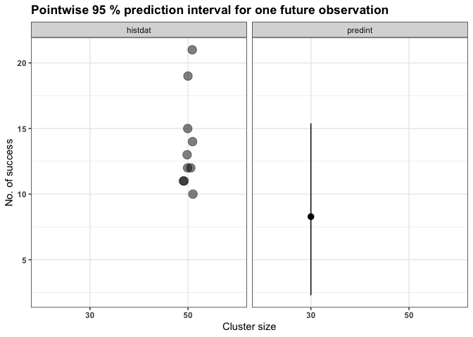
Menssen, M., Schaarschmidt, F.: Prediction intervals for all of M future observations based on linear random effects models. Statistica Neerlandica. 2022.
Menssen M, Schaarschmidt F.: Prediction intervals for overdispersed binomial data with application to historical controls. Statistics in Medicine. 2019;38:2652-2663.
NTP 2017: Tables of historical controls: pathology tables by route/vehicle., Accessed May 17, 2017.