ppsr - Predictive
Power Score![]()
![]()
ppsr is the R implementation of the Predictive
Power Score (PPS).
The PPS is an asymmetric, data-type-agnostic score that can detect linear or non-linear relationships between two variables. The score ranges from 0 (no predictive power) to 1 (perfect predictive power).
The general concept of PPS is useful for data exploration purposes, in the same way correlation analysis is. You can read more about the (dis)advantages of using PPS in this blog post.
You can install the latest stable version of ppsr from
CRAN:
install.packages('ppsr')Not all recent features and bugfixes may be included in the CRAN release.
Instead, you might want to download the most recent developmental
version of ppsr from Github:
# install.packages('devtools') # Install devtools if needed
devtools::install_github('https://github.com/paulvanderlaken/ppsr')PPS represents a framework for evaluating predictive validity.
There is not one single way of computing a predictive power score, but rather there are many different ways.
You can select different machine learning algorithms, their associated parameters, cross-validation schemes, and/or model evaluation metrics. Each of these design decisions will affect your model’s predictive performance and, in turn, affect the resulting predictive power score you compute.
Hence, you can compute many different PPS for any given predictor and target variable.
For example, the PPS computed with a decision tree regression model…
ppsr::score(iris, x = 'Sepal.Length', y = 'Petal.Length', algorithm = 'tree')[['pps']]
#> [1] 0.6160836
…will differ from the PPS computed with a simple linear regression model.
ppsr::score(iris, x = 'Sepal.Length', y = 'Petal.Length', algorithm = 'glm')[['pps']]
#> [1] 0.5441131The ppsr package has four main functions to compute
PPS:
score() computes an x-y PPSscore_predictors() computes all X-y PPSscore_df() computes all X-Y PPSscore_matrix() computes all X-Y PPS, and shows them in
a matrixwhere x and y represent an individual
predictor/target, and X and Y represent all
predictors/targets in a given dataset.
score() computes the PPS for a single target and
predictor
ppsr::score(iris, x = 'Sepal.Length', y = 'Petal.Length')
#> $x
#> [1] "Sepal.Length"
#>
#> $y
#> [1] "Petal.Length"
#>
#> $result_type
#> [1] "predictive power score"
#>
#> $pps
#> [1] 0.6160836
#>
#> $metric
#> [1] "MAE"
#>
#> $baseline_score
#> [1] 1.571967
#>
#> $model_score
#> [1] 0.5971445
#>
#> $cv_folds
#> [1] 5
#>
#> $seed
#> [1] 1
#>
#> $algorithm
#> [1] "tree"
#>
#> $model_type
#> [1] "regression"
score_predictors() computes all PPSs for a single target
using all predictors in a dataframe
ppsr::score_predictors(df = iris, y = 'Species')
#>              x       y                       result_type       pps      metric
#> 1 Sepal.Length Species            predictive power score 0.5591864 F1_weighted
#> 2  Sepal.Width Species            predictive power score 0.3134401 F1_weighted
#> 3 Petal.Length Species            predictive power score 0.9167580 F1_weighted
#> 4  Petal.Width Species            predictive power score 0.9398532 F1_weighted
#> 5      Species Species predictor and target are the same 1.0000000        <NA>
#>   baseline_score model_score cv_folds seed algorithm     model_type
#> 1      0.3176487   0.7028029        5    1      tree classification
#> 2      0.3176487   0.5377587        5    1      tree classification
#> 3      0.3176487   0.9404972        5    1      tree classification
#> 4      0.3176487   0.9599148        5    1      tree classification
#> 5             NA          NA       NA   NA      <NA>           <NA>
score_df() computes all PPSs for every target-predictor
combination in a dataframe
ppsr::score_df(df = iris)
#>               x            y                       result_type        pps
#> 1  Sepal.Length Sepal.Length predictor and target are the same 1.00000000
#> 2   Sepal.Width Sepal.Length            predictive power score 0.04632352
#> 3  Petal.Length Sepal.Length            predictive power score 0.54913985
#> 4   Petal.Width Sepal.Length            predictive power score 0.41276679
#> 5       Species Sepal.Length            predictive power score 0.40754872
#> 6  Sepal.Length  Sepal.Width            predictive power score 0.06790301
#> 7   Sepal.Width  Sepal.Width predictor and target are the same 1.00000000
#> 8  Petal.Length  Sepal.Width            predictive power score 0.23769911
#> 9   Petal.Width  Sepal.Width            predictive power score 0.21746588
#> 10      Species  Sepal.Width            predictive power score 0.20128762
#> 11 Sepal.Length Petal.Length            predictive power score 0.61608360
#> 12  Sepal.Width Petal.Length            predictive power score 0.24263851
#> 13 Petal.Length Petal.Length predictor and target are the same 1.00000000
#> 14  Petal.Width Petal.Length            predictive power score 0.79175121
#> 15      Species Petal.Length            predictive power score 0.79049070
#> 16 Sepal.Length  Petal.Width            predictive power score 0.48735314
#> 17  Sepal.Width  Petal.Width            predictive power score 0.20124105
#> 18 Petal.Length  Petal.Width            predictive power score 0.74378445
#> 19  Petal.Width  Petal.Width predictor and target are the same 1.00000000
#> 20      Species  Petal.Width            predictive power score 0.75611126
#> 21 Sepal.Length      Species            predictive power score 0.55918638
#> 22  Sepal.Width      Species            predictive power score 0.31344008
#> 23 Petal.Length      Species            predictive power score 0.91675800
#> 24  Petal.Width      Species            predictive power score 0.93985320
#> 25      Species      Species predictor and target are the same 1.00000000
#>         metric baseline_score model_score cv_folds seed algorithm
#> 1         <NA>             NA          NA       NA   NA      <NA>
#> 2          MAE      0.6893222   0.6620058        5    1      tree
#> 3          MAE      0.6893222   0.3100867        5    1      tree
#> 4          MAE      0.6893222   0.4040123        5    1      tree
#> 5          MAE      0.6893222   0.4076661        5    1      tree
#> 6          MAE      0.3372222   0.3184796        5    1      tree
#> 7         <NA>             NA          NA       NA   NA      <NA>
#> 8          MAE      0.3372222   0.2564258        5    1      tree
#> 9          MAE      0.3372222   0.2631636        5    1      tree
#> 10         MAE      0.3372222   0.2677963        5    1      tree
#> 11         MAE      1.5719667   0.5971445        5    1      tree
#> 12         MAE      1.5719667   1.1945031        5    1      tree
#> 13        <NA>             NA          NA       NA   NA      <NA>
#> 14         MAE      1.5719667   0.3265152        5    1      tree
#> 15         MAE      1.5719667   0.3280552        5    1      tree
#> 16         MAE      0.6623556   0.3377682        5    1      tree
#> 17         MAE      0.6623556   0.5315834        5    1      tree
#> 18         MAE      0.6623556   0.1684906        5    1      tree
#> 19        <NA>             NA          NA       NA   NA      <NA>
#> 20         MAE      0.6623556   0.1608119        5    1      tree
#> 21 F1_weighted      0.3176487   0.7028029        5    1      tree
#> 22 F1_weighted      0.3176487   0.5377587        5    1      tree
#> 23 F1_weighted      0.3176487   0.9404972        5    1      tree
#> 24 F1_weighted      0.3176487   0.9599148        5    1      tree
#> 25        <NA>             NA          NA       NA   NA      <NA>
#>        model_type
#> 1            <NA>
#> 2      regression
#> 3      regression
#> 4      regression
#> 5      regression
#> 6      regression
#> 7            <NA>
#> 8      regression
#> 9      regression
#> 10     regression
#> 11     regression
#> 12     regression
#> 13           <NA>
#> 14     regression
#> 15     regression
#> 16     regression
#> 17     regression
#> 18     regression
#> 19           <NA>
#> 20     regression
#> 21 classification
#> 22 classification
#> 23 classification
#> 24 classification
#> 25           <NA>
score_df() computes all PPSs for every target-predictor
combination in a dataframe, but returns only the scores arranged in a
neat matrix, like the familiar correlation matrix
ppsr::score_matrix(df = iris)
#>              Sepal.Length Sepal.Width Petal.Length Petal.Width   Species
#> Sepal.Length   1.00000000  0.04632352    0.5491398   0.4127668 0.4075487
#> Sepal.Width    0.06790301  1.00000000    0.2376991   0.2174659 0.2012876
#> Petal.Length   0.61608360  0.24263851    1.0000000   0.7917512 0.7904907
#> Petal.Width    0.48735314  0.20124105    0.7437845   1.0000000 0.7561113
#> Species        0.55918638  0.31344008    0.9167580   0.9398532 1.0000000
Currently, the ppsr package computes PPS by default
using…
rpart
package, wrapped by parsnipYou can call the available_algorithms() and
available_evaluation_metrics() functions to see what
alternative settings are supported.
Note that the calculated PPS reflects the
out-of-sample predictive validity when more than a
single cross-validation is used. If you prefer to look at in-sample
scores, you can set cv_folds = 1. Note that in such cases
overfitting can become an issue, particularly with the more flexible
algorithms.
Subsequently, there are three main functions that wrap around these
computational functions to help you visualize your PPS using
ggplot2:
visualize_pps() produces a barplot of all X-y PPS, or a
heatmap of all X-Y PPSvisualize_correlations() produces a heatmap of all X-Y
correlationsvisualize_both() produces the two heatmaps of all X-Y
PPS and correlations side-by-sideIf you specify a target variable (y) in
visualize_pps(), you get a barplot of its predictors.
ppsr::visualize_pps(df = iris, y = 'Species')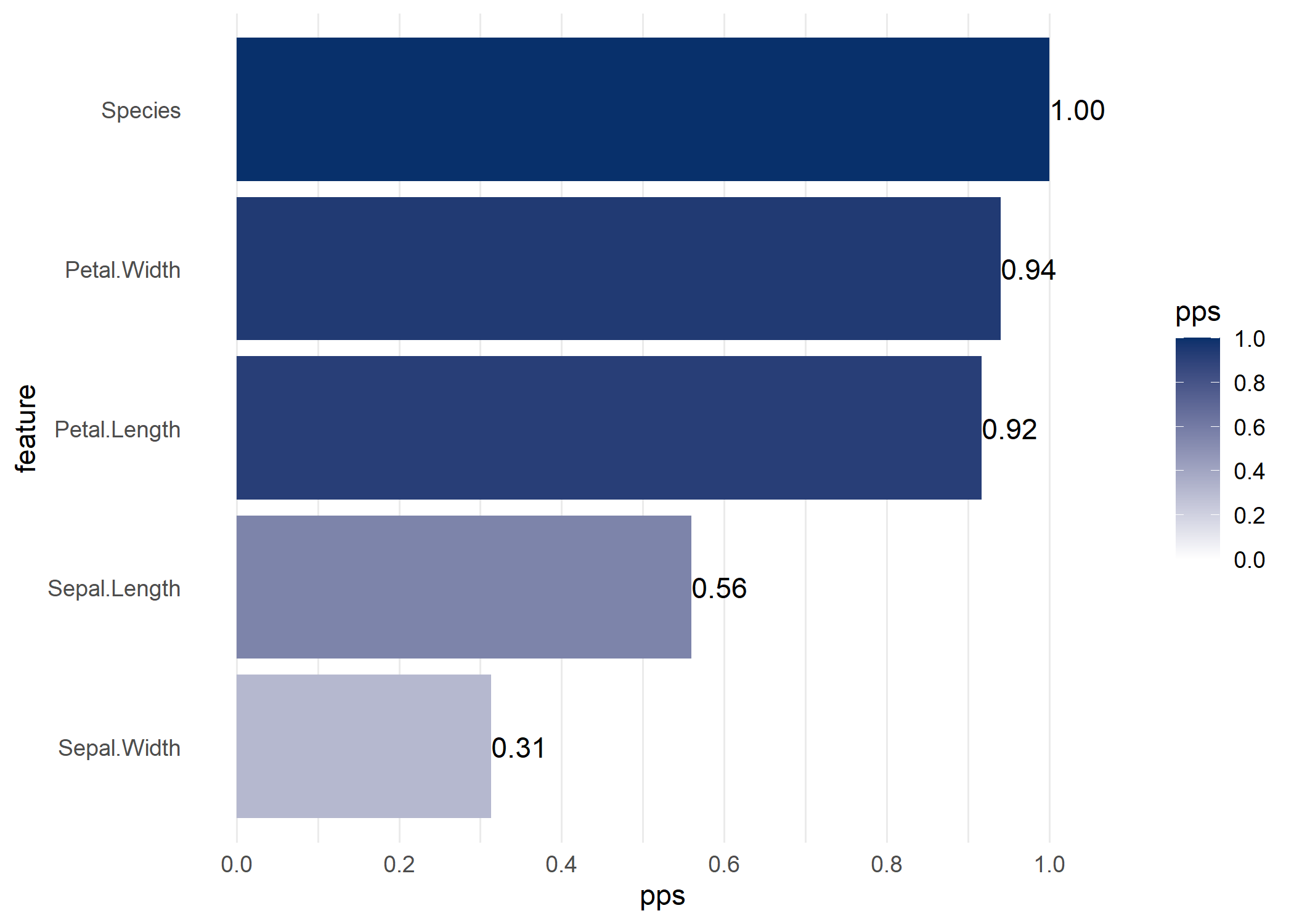
If you do not specify a target variable in
visualize_pps(), you get the PPS matrix visualized as a
heatmap.
ppsr::visualize_pps(df = iris)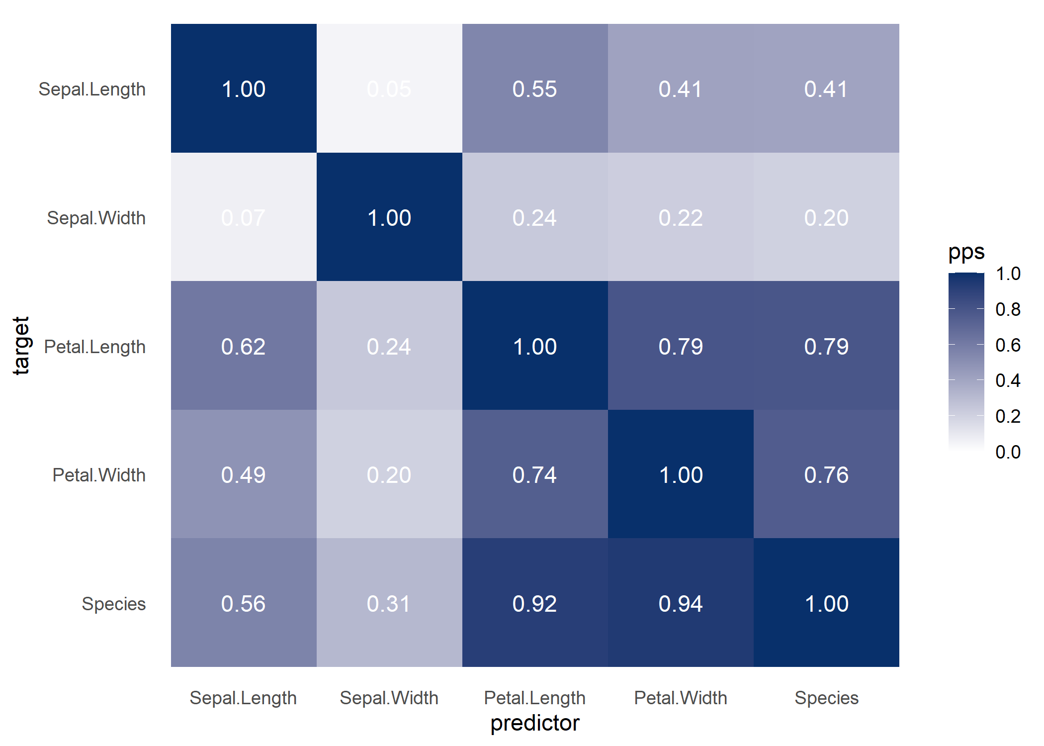
Some users might find it useful to look at a correlation matrix for comparison.
ppsr::visualize_correlations(df = iris)
With visualize_both you generate the PPS and correlation
matrices side-by-side, for easy comparison.
ppsr::visualize_both(df = iris)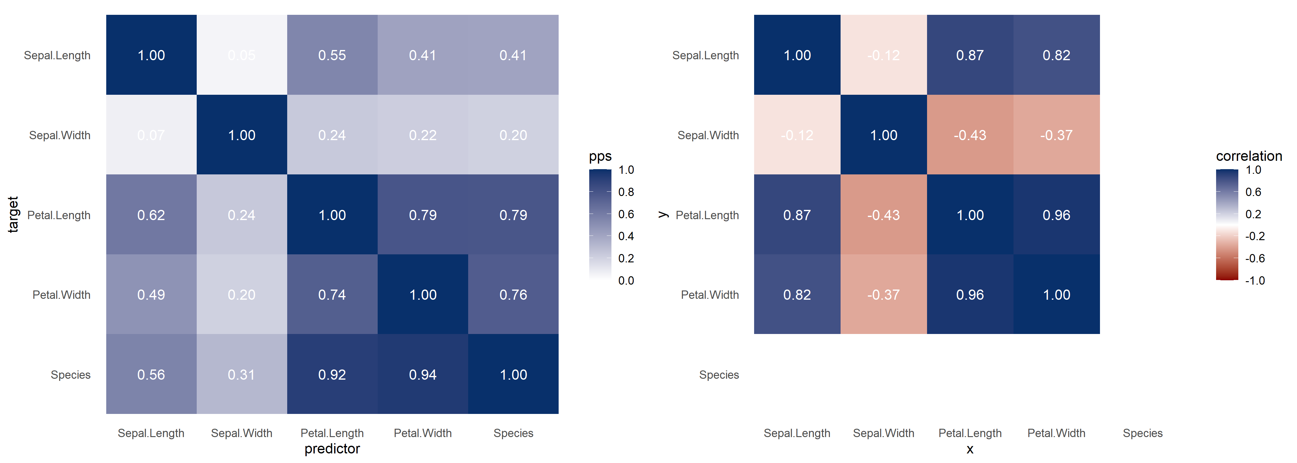
You can change the colors of the visualizations using the functions arguments. There are also arguments to change the color of the text scores.
Furthermore, the functions return ggplot2 objects, so
that you can easily change the theme and other settings.
ppsr::visualize_pps(df = iris,
                    color_value_high = 'red',
                    color_value_low = 'yellow',
                    color_text = 'black') +
  ggplot2::theme_classic() +
  ggplot2::theme(plot.background = ggplot2::element_rect(fill = "lightgrey")) +
  ggplot2::theme(title = ggplot2::element_text(size = 15)) +
  ggplot2::labs(title = 'Add your own title',
                subtitle = 'Maybe an informative subtitle',
                caption = 'Did you know ggplot2 includes captions?',
                x = 'You could call this\nthe independent variable\nas well')
The number of predictive models that one needs to build in order to fill the PPS matrix belonging to a dataframe increases exponentially with every new column in that dataframe.
For traditional correlation analyses, this is not a problem. Yet, with more computation-intensive algorithms, with many train-test splits, and with large or high-dimensional datasets, it can take a decent amount of time to build all the predictive models and derive their PPSs.
One way to speed matters up is to use the
ppsr::score_predictors() function and focus on predicting
only the target/dependent variable you are most interested in.
Yet, since version 0.0.1, all ppsr::score_*
and pssr::visualize_* functions now take in two arguments
that facilitate parallel computing. You can parallelize
ppsr’s computations by setting the do_parallel
argument to TRUE. If done so, a cluster will be created
using the parallel package. By default, this cluster will
use the maximum number of cores (see
parallel::detectCores()) minus 1.
However, with the second argument – n_cores – you can
manually specify the number of cores you want ppsr to
use.
Examples:
ppsr::score_df(df = mtcars, do_parallel = TRUE)ppsr::visualize_pps(df = iris, do_parallel = TRUE, n_cores = 2)The PPS is a normalized score that ranges from 0 (no predictive power) to 1 (perfect predictive power).
The normalization occurs by comparing how well we are able to predict
the values of a target variable (y) using the
values of a predictor variable (x), respective to
two benchmarks: a perfect prediction, and a naive
prediction
The perfect prediction can be theoretically derived. A perfect regression model produces no error (=0.0), whereas a perfect classification model results in 100% accuracy, recall, et cetera (=1.0).
The naive prediction is derived empirically. A naive
regression model is simulated by predicting the mean
y value for all observations. This is similar to how
R-squared is calculated. A naive classification model is
simulated by taking the best among two models: one predicting the modal
y class, and one predicting random y classes
for all observations.
Whenever we train an “informed” model to predict y using
x, we can assess how well it performs by comparing it to
these two benchmarks.
Suppose we train a regression model, and its mean average error (MAE) is 0.10. Suppose the naive model resulted in an MAE of 0.40. We know the perfect model would produce no error, which means an MAE of 0.0.
With these three scores, we can normalize the performance of our informed regression model by interpolating its score between the perfect and the naive benchmarks. In this case, our model’s performance lies about 1/4th of the way from the perfect model, and 3/4ths of the way from the naive model. In other words, our model’s predictive power score is 75%: it produced 75% less error than the naive baseline, and was only 25% short of perfect predictions.
Using such normalized scores for model performance allows us to easily interpret how much better our models are as compared to a naive baseline. Moreover, such normalized scores allow us to compare and contrast different modeling approaches, in terms of the algorithms, the target’s data type, the evaluation metrics, and any other settings used.
The main use of PPS is as a tool for data exploration. It trains out-of-the-box machine learning models to assess the predictive relations in your dataset.
However, this PPS is quite a “quick and dirty” approach. The trained
models are not at all tailored to your specific
regression/classification problem. For example, it could be that you get
many PPSs of 0 with the default settings. A known issue is that the
default decision tree often does not find valuable splits and reverts to
predicting the mean y value found at its root. Here, it
could help to try calculating PPS with different settings (e.g.,
algorithm = 'glm').
At other times, predictive relationships may rely on a combination of variables (i.e. interaction/moderation). These are not captured by the PPS calculations, which consider only univariate relations. PPS is simply not suited for capturing such complexities. In these cases, it might be more interesting to train models on all your features simultaneously and turn to concepts like feature/variable importance, partial dependency, conditional expectations, accumulated local effects, and others.
In general, the PPS should not be considered more than a fast and easy tool to finding starting points for further, in-depth analysis. Keep in mind that you can build much better predictive models than the default PPS functions if you tailor your modeling efforts to your specific data context.
PPS is a relatively young concept, and likewise the ppsr
package is still under development. If you spot any bugs or potential
improvements, please raise an issue or submit a pull request.
On the developmental agenda are currently:
This R package was inspired by 8080labs’ Python package ppscore.
The same 8080labs also developed an earlier, unfinished R implementation of PPS.
Read more about the big ideas behind PPS in this blog post.