The {peruse} package is aimed at making it easier to generate irregular sequences that are difficult to generate with existing tools.
The heart of {peruse} is the S3 class
Iterator. An Iterator allows the user to write
an arbitrary R expression that returns the next element of a sequence of
R objects. It then saves the state of the Iterator, meaning
the next time evaluation is invoked, the initial state will be the
result of the previous iteration. This is most useful for generating
recursive sequences, those where each iteration depends on previous
ones.
The package also provides a simple, tidy API for set building,
allowing the user to generate a set consisting of the elements of a
vector that meet specific criteria. This can either return a vector
consisting of all the chosen elements or it can return an
Iterator that lazily generates the chosen elements.
At the end of this document, there is a tutorial for metaprogramming
(that is, programmatically generating code) with
Iterators.
You can install the released version of peruse from CRAN with:
install.packages("peruse")And the development version from GitHub with:
# install.packages("devtools")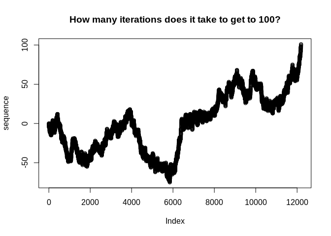
devtools::install_github("jacgoldsm/peruse")Suppose we want to investigate the question of how many trials it takes for a random walk with drift to reach a given threshold. We know that this would follow a Negative Binomial distribution, but how could we use the Iterator to look at this empirically in a way that easily allows us to adjust the drift term and see how the result changes? We might do something like this:
p_success <- 0.5
threshold <- 100


iter <- Iterator({
          set.seed(seeds[.iter])
          n <- n + sample(c(1,-1), 1, prob = c(p_success, 1 - p_success))
        },
        list(n = 0, seeds = 1000:1e5),
        n)
sequence <- yield_while(iter, n <= threshold)

plot(sequence, main = "How many iterations does it take to get to 100?")
How would we apply this same function to a grid of probabilities? We could do something like this:
probs <- seq(0.5,0.95, by = 0.01)
num_iter <- rep(NA, length(probs))
threshold <- 20
seeds <- 1000:1e6


for (i in seq_along(probs)) {
  iter <- Iterator({
           set.seed(seeds[.iter])
           n <- n + sample(c(1,-1), 1, prob = c(!! probs[i], 1 - !! probs[i]))
          },
          list(n = 0),
          yield = n)

  num_iter[i] <- length(yield_while(iter, n <= threshold))
}

plot(x = probs,
     y = log(num_iter),
     main = "Probability of Success vs How long it takes to get to 20 (Log Scale)",
     xlab = "Probability of Success",
     ylab = "Log Number of Iterations")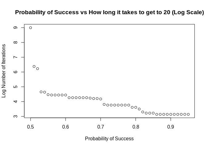
Alternatively, using functional programming:
make <- function(p) {
  iter <- Iterator({
    set.seed(seeds[.iter])
    n <- n + sample(c(1,-1), 1, prob = c(!! p, 1 - !! p))
  },
  list(n = 0),
  yield = n)

  length(yield_while(iter, n <= threshold))
}

num_iter <- sapply(seq(0.5,0.95, by = 0.01), make)
This illustrates a few useful features of Iterators:
We can use environment variables in either our expression or our
while condition to represent constants. In this case,
threshold doesn’t change between iterations or between
parameters. If you are creating many Iterators, it can be
faster to use environment variables, since you don’t have to make a new
object for each new Iterator.
We can use the forcing operators from {rlang}
(!!) to force evaluation of arguments in place, in this
case substituting the expression of probs[i] with
the value of probs[i] (see the end of this
document for a tutorial on metaprogramming with
Iterators).
We can refer to the current iteration number in
yield_while(), yield_more(), or their silent
variants with the variable .iter.
A Collatz sequence is a particular sequence of natural numbers that
mathematicians think always reaches 1 at some point, no matter the
starting point. We can’t prove that one way or the other, but we can
create an Iterator that lazily generates a Collatz sequence
until it reaches 1:
library(peruse)

# Collatz generator starting at 50
collatz <- Iterator({
             if (n %% 2 == 0) n <- n / 2 else n <- n*3 + 1
           },
           initial = list(n = 50),
           yield = n)

yield_while(collatz, n != 1L)
#>  [1] 25 76 38 19 58 29 88 44 22 11 34 17 52 26 13 40 20 10  5 16  8  4  2  1
Random Walks, with or without drift, are one of the most commonly used type of stochastic processes. How can we simulate one with {peruse}?
rwd <- Iterator({
         n <- n + sample(c(-1L, 1L), size = 1L, prob = c(0.25, 0.75))
       },
       initial = list(n = 0),
       yield = n)


Value <- yield_while(rwd, n != 50L & n != -50L)

plot(Value, main = "The Value of the Iterator after a Given Number of Iterations")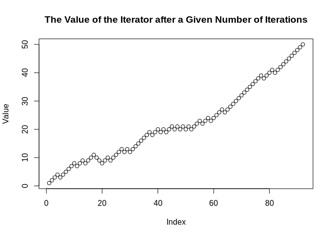
Here, we can see that seq gets to 50 after
about 100 iterations when it is weighted 3:1
odds in favor of adding 1 over adding -1 to
the prior value.
Helper functions yield_more(),
yield_while(), move_more(), and
move_while() behave mostly like syntactic sugar for
explicit loops. So,
it <- Iterator(x <- x + 1L, list(x = 0), x)
it2 <- clone(it)
x <- numeric(100)
for (i in 1:100) {
  x[i] <- yield_next(it)
}
will give the same result as
y <- yield_more(it2, 100)However, doing it the latter way is significantly more efficient than
the former. This is because a lot of the overhead only needs to be done
once per call to yield. That means that a lot less has to
be done on every iteration when you explicitly call
yield_more().
This is even more true with yield_while(). Pretend we
don’t know how long this Iterator will take to reach
10,000. Doing something like:
x <- numeric()
while (it$initial$x < 10000) {
  x <- c(x, yield_next(it))
}
is very inefficient because it requires reallocating the vector on every iteration. On the other hand, the following is both easier to read and much more efficient:
y <- yield_while(it2, x < 10000)Internally, yield_while() uses an efficient algorithm
for resizing the result in linear amortized time. As a result, it will
evaluate much faster.
How about generating all the prime numbers between 1 and
100? We can easily do that with the set-builder API:
2:100 %>%
  that_for_all(range(2, .x)) %>%
  we_have(~.x %% .y)
#>  [1]  2  3  5  7 11 13 17 19 23 29 31 37 41 43 47 53 59 61 67 71 73 79 83 89 97
In the equation, we can reference the left-hand side of the equation
with the positional variable .x, and the right-hand side
(that is, the argument in that_for_all()) with
.y. The equation can be anything recognized as a function
by rlang::as_function().
But how about if we want to generate the first 100 prime numbers? We don’t know the range of values this should fall in (well, mathematicians do), so we can use laziness to our advantage:
primes <- 2:10000 %>%
            that_for_all(range(2, .x)) %>%
            we_have(~.x %% .y, "Iterator")

primes_2 <- clone(primes)
The first prime number is
yield_next(primes_2)
#> [1] 2
And the first 100 are:
sequence <- yield_more(primes, 100)
sequence
#>   [1]   2   3   5   7  11  13  17  19  23  29  31  37  41  43  47  53  59  61
#>  [19]  67  71  73  79  83  89  97 101 103 107 109 113 127 131 137 139 149 151
#>  [37] 157 163 167 173 179 181 191 193 197 199 211 223 227 229 233 239 241 251
#>  [55] 257 263 269 271 277 281 283 293 307 311 313 317 331 337 347 349 353 359
#>  [73] 367 373 379 383 389 397 401 409 419 421 431 433 439 443 449 457 461 463
#>  [91] 467 479 487 491 499 503 509 521 523 541
Here, we use clone() to create an identical
Iterator to primes that can be modified
separately.
clone() also carries optional arguments that override
the $initial parameters in the old Iterator.
For example,
it <- Iterator({m <- m + n}, list(m = 0, n = 1), m)
it2 <- clone(it, n = 5)
yield_next(it)
#> [1] 1
yield_next(it2)
#> [1] 5
Here, we overrode n = 1 in it with
n = 5 in it2.
Iterators that are created from set comprehension have
several utilities:
Refer to the vector .x with the variable
.x_vector
Refer to the current index of .x_vector with
.i (not to be confused with .iter).
Here is an example of putting those together to yield to the end of the sequence:
primes_100 <- 2:100 %>%
              that_for_all(range(2, .x)) %>%
              we_have(~.x %% .y, "Iterator")

yield_while(primes_100, .x_vector[.i] <= 100)
#> (Note: result has reached end of sequence)
#>  [1]  2  3  5  7 11 13 17 19 23 29 31 37 41 43 47 53 59 61 67 71 73 79 83 89 97
As you can see, the sequence terminates with a message that the end has been reached.
In reality, the sequence will terminate at the end anyway, so you can generate the whole sequence like this:
primes_100 <- 2:100 %>%
              that_for_all(range(2, .x)) %>%
              we_have(~.x %% .y, "Iterator")

yield_while(primes_100, T)
#> (Note: result has reached end of sequence)
#> [1] 2 3 5 7 11 13 17 19 23 29 31 37 41 43 47 53 59 61 67 71 73 79 83 89 97Set comprehension does not specially handle missing values. All the
elements of set .x will be compared with all the elements
of set .y by formula, and the value of
.x will be included if and only if the condition returns
TRUE. If the comparison returns NA, the
expression will terminate with an error.
Be aware of two things: First, expressions like
NA == NA, NA > NA, and
NA <= NA return NA. Second, expressions of
the form if (NA) action are illegal and will result in an
error.
As a result, an expression like this will not work:
c(2:20, NA_integer_) %>% that_for_all(range(2, .x)) %>% we_have(~ .x %% .y)In fact, this will fail for two reasons: range(2, .x)
will not work when .x is NA, and the
comparison if (NA %% 2) will also not work.
Normally, you will want to drop NA values from your
vectors before using set comprehension. If you are careful, you can
write valid code with NAs, but it will be very painful by
comparison:
c(2:20, NA_integer_) %>%
  that_for_all(if (is.na(.x)) NA else range(2, .x)) %>%
  we_have(~ is.na(.x) || .x %% .y)
#> [1]  2  3  5  7 11 13 17 19 NA
Here, we avoid range(2, NA) with our conditional, and
avoid having NA in the if statement in
we_have() by making sure to return TRUE when
.x is missing.
IteratorsIterators are designed to be flexible, almost as
flexible as ordinary R functions. They are also designed to be tidy,
using tools from the “Tidyverse” family of R extensions. Unfortunately,
those goals are not entirely compatible when it comes to
metaprogramming, leading to a sort of “semi-tidy” evaluation. Use these
examples as a reference for programmatically generating
Iterator expressions.
In almost all cases, the environment in which an Iterator is made
does not effect its execution; rather, the environment from which
yield_next() or its cousins is called determines
evaluation. In this way, it is similar to ordinary R functions. The one
small exception will be detailed at the end.
Use !! to force evaluation of names, just like you would
in dplyr or any Tidyverse function:
p <- 0.5
i <- Iterator({x <- x + !! p}, list(x = 0), x)
yield_more(i, 5)
#> [1] 0.5 1.0 1.5 2.0 2.5
There is no built-in mechanism to force evaluation of names in the
$initial list, but you can use tools like
rlang::list2() to do so. $initial can be
anything coercible to list.
p <- 0.1
x <- as.symbol("my_var")
i <- Iterator({!! x <- !! x + !! p}, rlang::list2(!! x := 0), !! x)
yield_more(i, 5)
#> [1] 0.1 0.2 0.3 0.4 0.5
Note the use of the “walrus” operator (:=) to assign
names in rlang::list2(), see the documentation in
rlang::nse-force() for more details.
Function arguments are a special data structure in R. They really
represent up to three different things: the name given to the argument
in the function, possibly the name of the argument when the function is
called if it is named, and the value of the argument passed to the
function. Since Iterators don’t use quosures (because they
work independently of the environment where they are created), you can’t
use {{ }} to force-defuse expressions.
To get a variable name from a parameter name,
substitute() the variable at the beginning.
If you want the value of the variable, just leave it be.
Then use the bang-bang (!!) operator to add all of them
to the Iterator:
make_random_walk_with_drift <- function(drift, variable) {
  variable <- substitute(variable)  # creates a variable whose value is x
  Iterator({
    !! variable <- !! variable + sample(c(-1,1), 1, TRUE, c(!! drift, 1 - !! drift))
              },
    initial = rlang::list2(!! variable := 0), !! variable)
}

yield_more(make_random_walk_with_drift(0.5, x), 5)
#> [1] 1 2 1 0 -1Since Iterators don’t use data masks, they don’t have
.data and .env pronouns. If you have a
variable in iter$initial and a variable with the same name
in your global environment, just force immediate evaluation of the
environment variable with !!.
Ordinarily, Iterators work independently from the
environment in which they were created. The one exception is when an
Iterator is created from the template,
iterator <- .x %>% expression_with_.x %>% we_have(formula, "Iterator")the variable expression_with_.x is turned into a
quosure. That means that it will always be evaluated in the environment
where iterator was made.
For a concrete example, consider:
offset <- 2
it <- 2:100 %>% that_for_all(range(offset, .x)) %>% we_have(~ .x %% .y, "Iterator")
 fun <- function() {
  offset <- 3
  yield_while(it, !.finished) # print the whole sequence
 }

 fun()
#> (Note: result has reached end of sequence)
#>  [1]  2  3  5  7 11 13 17 19 23 29 31 37 41 43 47 53 59 61 67 71 73 79 83 89 97
We can see that the code does not select elements that are divisible
by 2 but not any other numbers, as would be the case with offset equal
to three. Our expression range(offset, .x) is evaluated in
the global environment, not in the execution environment of
fun().
This software contains a modified version of a small piece of code
from the purrr package, by Hadley Wickham, Lionel Henry,
and RStudio, freely available under the MIT License.