
The personalized2part package implements the methodology
of Huling, Smith, and Chen (2020), which allows for subgroup
identification for semi-continuous outcomes by estimating individualized
treatment rules. It uses a two part modeling (or hurdle modeling)
framework to handle semi-continuous data by modeling separately the
positive part of the outcome and an indicator of whether each outcome is
positive, but still results in a single treatment rule. High dimensional
data is handled with a cooperative lasso penalty, which encourages the
coefficients in the two models to have the same sign.
You can install the development version from GitHub with:
# install.packages("devtools")
devtools::install_github("jaredhuling/personalized2part")This is a basic example which shows you how to solve a common problem:
library(personalized2part)Simulate semicontinuous data with a heterogeneous treatment effect:
set.seed(1)
dat <- sim_semicontinuous_data(n.obs = 300, n.vars = 50)

x   <- dat$x
y   <- dat$y
trt <- dat$trt
Use the built-in function create.propensity.function
from the personalized
package to construct a function that fits a propensity score model using
10-fold cross fitting:
propens_func <- create.propensity.function(crossfit = TRUE,
                                           nfolds.crossfit = 10,
                                           cv.glmnet.args = list(type.measure = "auc"))
Use the built-in function create.augmentation.function
from the personalized
package to construct outcome augmentation functions for the zero part
model using 10-fold cross fitting:
aug_func_binary <- create.augmentation.function(family = "binomial",
                                                crossfit = TRUE,
                                                nfolds.crossfit = 10,
                                                cv.glmnet.args = list(type.measure = "auc"))
Use the built-in function HDtweedie_kfold_aug from the
personalized2part package to construct outcome augmentation functions
for the positive part model using 10-fold cross fitting using a
penalized gamma regression model:
aug_func_positive <- function(x, y, trt)
{
        HDtweedie_kfold_aug(x, y, trt, K = 10, p = 2,
                            interactions = TRUE)
}
fitted_2part_subgrp_model <- fit_subgroup_2part(x, y, trt,
propensity.func = propens_func,
propensity.func.positive = propens_func,
augment.func.zero = aug_func_binary,
augment.func.positive = aug_func_positive)
## the model print display takes the same form as fitted models from
## the personalized package
fitted_2part_subgrp_model
#> family: 2part
#> loss: 2part
#> method:
#> cutpoint: 1
#> propensity
#> function: propensity.func
#>
#> benefit score: f(x),
#> Trt recom = 1*I(f(x)>c)+0*I(f(x)<=c) where c is 'cutpoint'
#>
#> Average Outcomes:
#> Recommended 0 Recommended 1
#> Received 0 7.1015 (n = 93) 0.3277 (n = 49)
#> Received 1 0.4653 (n = 47) 6.4159 (n = 111)
#>
#> Treatment effects conditional on subgroups:
#> Est of E[Y|T=0,Recom=0]-E[Y|T=/=0,Recom=0]
#> 6.6363 (n = 140)
#> Est of E[Y|T=1,Recom=1]-E[Y|T=/=1,Recom=1]
#> 6.0882 (n = 160)
#>
#> NOTE: The above average outcomes are biased estimates of
#> the expected outcomes conditional on subgroups.
#> Use 'validate.subgroup()' to obtain unbiased estimates.
#>
#> ---------------------------------------------------
#>
#> Benefit score quantiles (f(X) for 1 vs 0):
#> 0% 25% 50% 75% 100%
#> 4.414e-03 3.333e-01 1.220e+00 5.312e+00 2.131e+02
#>
#> ---------------------------------------------------
#>
#> Summary of individual treatment effects:
#> E[Y|T=1, X] / E[Y|T=0, X]
#>
#> Note: for survival outcomes, the above ratio is
#> E[g(Y)|T=1, X] / E[g(Y)|T=0, X],
#> where g() is a monotone increasing function of Y,
#> the survival time
#>
#> Min. 1st Qu. Median Mean 3rd Qu. Max.
#> 0.00441 0.33333 1.21976 10.03182 5.31193 213.08937We can plot the coefficient curves for the two models as the following:
par(mfrow = c(1,2))
plot(fitted_2part_subgrp_model$model$hd2part.fit, "zero")
plot(fitted_2part_subgrp_model$model$hd2part.fit, "positive")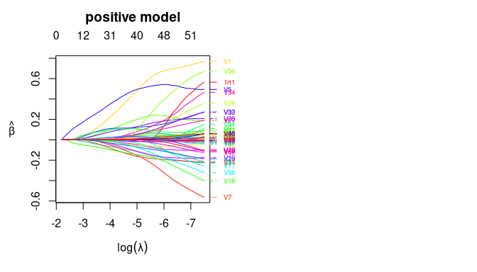
Now evaluate value function on test set based on the estimated individualized treatment rule and compare with average outcome (a value function larger than the average outcome means that the ITR results in better outcomes than standard practice). The predict function returns predicted values for the heterogeneous treatment effect in terms of the risk ratio (E[Y|X,T=1] / E[Y|X,T=-1]), so greater than 1 means the treatment is beneficial (if larger outcomes are preferred).
dat.test <- sim_semicontinuous_data(n.obs = 10000, n.vars = 50)

x.test   <- dat.test$x
y.test   <- dat.test$y

predicted_hte <- predict(fitted_2part_subgrp_model, x.test)

## estmated test set value function:
personalized2part:::computeValue(y.test, predicted_hte, dat.test$trt,
                                 pi.x = dat.test$pi.x, cutoff = 1)
#> [1] 4.708711

## average outcome in the test set:
mean(dat.test$y)
#> [1] 3.854057

# We can see that the estimated treatment rule results in better outcomes for the test set
Now let’s compare with simply using a squared error loss under the framework of Chen, et al (2017) to estimate an ITR:
fsm_log <- fit.subgroup(x, log(y+0.1), trt, propensity.func = propens_func,
                    augment.func = create.augmentation.function(family="gaussian"),
                    loss = "sq_loss_lasso")

fsm <- fit.subgroup(x, y, trt, propensity.func = propens_func,
                    augment.func = create.augmentation.function(family="gaussian"),
                    loss = "sq_loss_lasso")

pred_hte_sqloss_log <- predict(fsm_log, x.test)
pred_hte_sqloss <- predict(fsm, x.test)

## the value function is smaller than for the 2 part model
personalized2part:::computeValue(y.test, pred_hte_sqloss, dat.test$trt,
                                 pi.x = dat.test$pi.x, cutoff = 0)
#> [1] 1.763163

personalized2part:::computeValue(y.test, pred_hte_sqloss_log, dat.test$trt,
                                 pi.x = dat.test$pi.x, cutoff = 0)
#> [1] 4.172806[1] Huling J, Smith M, Chen G (2020). A two-part framework for estimating individualized treatment rules from semi-continuous outcomes. Journal of the American Statistical Association, in press.
[2] Chen S, Tian L, Cai T, Yu M (2017). A general statistical framework for subgroup identification and comparative treatment scoring. Biometrics, 73(4):1199-209.