![]()
Estimating sample size and statistical power is an essential part of a good study design. This package allows users to conduct power analysis based on Monte Carlo simulations in settings in which considerations of the correlations between predictors are important. It runs power analyses given a data generative model and an inference model. It can set up a data generative model that preserves dependence structures among variables given existing data (continuous, binary, or ordinal) or high-level descriptions of the associations. Users can generate power curves to assess the trade-offs between sample size, effect size, and power of a design.
This vignette presents tutorials and examples focusing on applications for environmental mixtures studies where predictors tend to be moderately to highly correlated. It easily interfaces with several existing and newly developed analysis strategies for assessing associations between exposures to mixtures and health outcomes. However, the package is sufficiently general to facilitate power simulations in a wide variety of settings.
And the development version from GitHub with:
# install.packages("devtools")
devtools::install_github("phuchonguyen/mpower")library(mpower)
library(dplyr)
library(magrittr)
library(tidyselect)
library(ggplot2)To do power analysis using Monte Carlo simulations, we’ll need:
A generative model for the predictors. The predictors can be
correlated and mixed-scaled. Use MixtureModel().
A generative model for the outcome that describes the “true”
relationships between the predictors and outcome. Use
OutcomeModel().
An inference model. Ideally, this would be the same as the
generative model for the outcome. However, in practice our model can at
best approximate the “true” predictor-outcome relationships. Use
InferenceModel().
A “significance” criterion and threshold for the inference model. For instance, the t-test in a linear regression has its p-value as the “significance” criterion, and a common threshold for statistical significance is p-value less than 0.05.
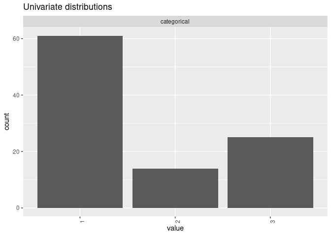
We can manually specify the joint distribution of the predictors using univariate marginal distributions and a guess of the correlation matrix. To create four moderately associated mixed-scaled predictors:
G <- diag(1, 4)
G[upper.tri(G)] <- 0.6
G[lower.tri(G)] <- 0.6
xmod <- mpower::MixtureModel(method = "cvine", G = G, m = 50,
    cvine_marginals = list(binary = "qbinom(size=1, prob=0.2)",
                           count = "qpois(lambda = 1)",
                           ordinal = "qmultinom(probs=c(0.6, 0.2, 0.2))",
                           categorical = "qmultinom(probs=c(0.6, 0.2, 0.2))"),
    cvine_dtypes = list(categorical = "factor"))
mpower::mplot(xmod)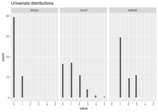
Since we want to create a power curve, we need to supply a list of outcome models with different “true” effect sizes:
ymod_list <- list(
  mpower::OutcomeModel(f = "1*binary + 1*I(categorical==1)", sigma = 1, family = "gaussian"),
  mpower::OutcomeModel(f = "0.5*binary + 0.5*I(categorical==1)", sigma = 1, family = "gaussian"),
  mpower::OutcomeModel(f = "0.2*binary + 0.2*I(categorical==1)", sigma = 1, family = "gaussian")
)We define an overall F-test for linear regression as the inference model and the p-value as the “significance” criterion:
# Define the ftest that returns a list of significance criteria
ftest <- function(y, x) {
  dat <- as.data.frame(cbind(y, x))
  lm_mod <- lm(y ~ ., data = dat)
  fstat <- summary.lm(lm_mod)$fstat
  fpval <- pf(fstat[1], fstat[2], fstat[3], lower.tail=F)
  names(fpval) <- "F-test"
  return(list(pval = fpval))
}
# define an InferenceModel using the F-test
imod <- mpower::InferenceModel(model = ftest, name = "F-test")We run power analysis for sample sizes 100 and 300 with 2 cores and 100 Monte Carlo simulations:
curve <- mpower::sim_curve(xmod, ymod_list, imod, s = 100,
                   n = c(100, 300), cores = 2)
We can get a table of summaries and a plot of the power:
curve_df <- mpower::summary(curve , crit = "pval", thres = 0.05, how = "lesser")
#>
#>  *** POWER CURVE ANALYSIS SUMMARY ***
#> Number of Monte Carlo simulations: 100
#> Number of observations in each simulation: 100 300
#> Data generating process estimated SNR (for each outcome model): 0.31 0.07 0.01
#> Inference model: F-test
#> Significance criterion: pval
#> Significance threshold: 0.05
#>
#> |       | power|   n|  snr|
#> |:------|-----:|---:|----:|
#> |F-test |  0.99| 100| 0.31|
#> |F-test |  0.48| 100| 0.07|
#> |F-test |  0.09| 100| 0.01|
#> |F-test |  1.00| 300| 0.31|
#> |F-test |  0.94| 300| 0.07|
#> |F-test | 0.27| 300| 0.01|mpower::plot_summary(curve , crit = "pval", thres = 0.05, how = "lesser")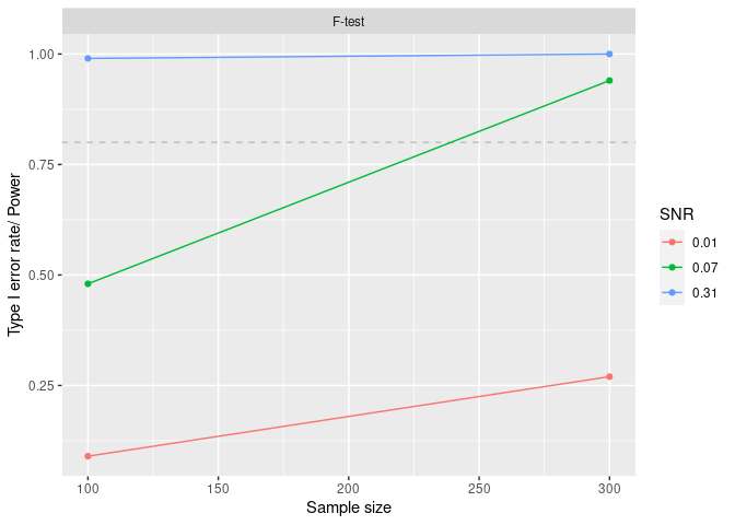
We can estimate a data generative model for the predictors if we have existing data on them. For example, here we use a copy of the NHANES data from the 2015-2016 and 2017-2018 cycles.
For an estimation model, all data must be in numeric form. Categorical variables should be converted to factors with numeric categories:
data("nhanes1518")
# preprocessing step
phthalates_names <- c("URXCNP", "URXCOP", "URXECP", "URXHIBP",
         "URXMBP", "URXMC1", "URXMCOH", "URXMEP", "URXMHBP", "URXMHH",
         "URXMHNC", "URXMHP", "URXMIB", "URXMNP", "URXMOH", "URXMZP")
covariates_names <- c("RIDAGEYR","INDHHIN2","BMXBMI","RIAGENDR")
# Get set of complete data only. Remaining 4800 obs.
nhanes_nona <- nhanes1518 %>%
  select(all_of(c(phthalates_names, covariates_names))) %>%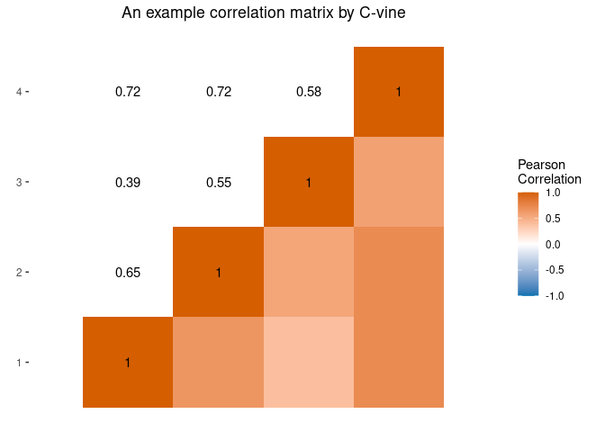
filter(complete.cases(.))We use a Bayesian semi-parametric Gaussian copula for this step. See
more in the R package sbgcop.
xmod <- mpower::MixtureModel(method = "estimation" , data = nhanes_nona,
sbg_args = list(nsamp = 1000))mplot(xmod, split=F)$corr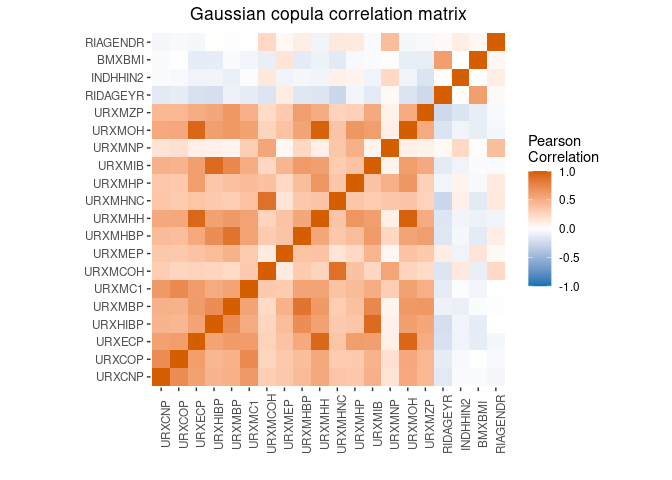
ymod <- mpower::OutcomeModel(sigma = 1, family = "gaussian",
                     f = "0.5*RIDAGEYR + 0.3*I(RIAGENDR==1) +
0.3*URXMHH + 0.2*URXMOH + 0.2*URXMHP")power <- mpower::sim_power(xmod, ymod, imod, s=1000, n=100, snr_iter=4800,
cores = 2, errorhandling = "stop") power_df <- mpower::summary(power , crit = "pval", thres = 0.05, how = "lesser")
#>
#> *** POWER ANALYSIS SUMMARY ***
#> Number of Monte Carlo simulations: 1000
#> Number of observations in each simulation: 100
#> Data generating process estimated SNR: 232.71
#> Inference model: F-test
#> Significance criterion: pval
#>
#> Significance threshold: 0.05
#>
#> | | power|
#> |:------|-----:|
#> |F-test | 1|In this example, we generate predictors by resampling of a large existing dataset. We load data from the R package NHANES and treat ordinal Education and HHIncome as continuous variables.
library(NHANES)
data("NHANES")
nhanes_demo <- NHANES %>%
  select(BMI, Education, HHIncome, HomeOwn, Poverty, Age) %>%
  filter(complete.cases(.)) %>%
  mutate(Education = case_when(Education == "8th Grade" ~ 1,
                               Education == "9 - 11th Grade" ~ 2,
                               Education == "High School" ~ 3,
                               Education == "Some College" ~ 4,
                               Education == "College Grad" ~ 5),
         HHIncome = case_when(HHIncome == "more 99999" ~ 12,
                              HHIncome == "75000-99999" ~ 11,
                              HHIncome == "65000-74999" ~ 10,
                              HHIncome == "55000-64999" ~ 9,
                              HHIncome == "45000-54999" ~ 8,
                              HHIncome == "35000-44999" ~ 7,
                              HHIncome == "25000-34999" ~ 6,
                              HHIncome == "20000-24999" ~ 5,
                              HHIncome == "15000-19999" ~ 4,
                              HHIncome == "10000-14999" ~ 3,
                              HHIncome == " 5000-9999" ~ 2,
                              HHIncome == " 0-4999" ~ 1))
xmod <- mpower::MixtureModel(method = "resampling", data = nhanes_demo %>% select(- BMI))We can generate outcomes from a previously fitted model.
lm_demo <- lm(BMI ~ Poverty*(poly(Age, 2) + HHIncome + HomeOwn + Education), data = nhanes_demo)
# wrapper function that takes a data frame x and returns a vector of outcome
f_demo <- function(x) {
  predict.lm(lm_demo, newdata = x)
}
ymod <- mpower::OutcomeModel(f = f_demo, family = "gaussian",
sigma = sigma(lm_demo))glm
modelWe need to give glm the family and formula inputs. See
documentation of glm for more options.
# pass the formula argument to glm()
imod <- mpower::InferenceModel(model = "glm", family = "gaussian",
    formula = y ~ Poverty*(poly(Age, 2) + HHIncome + HomeOwn + Education))
The model lm_demo is defined in the global environment,
outside the scope of the parallel processes. We need to pass
"lm_demo" to the cluster_export argument to
make sure the variable is defined while using parallelism.
curve <- mpower::sim_curve(xmod, ymod, imod,
    s = 200, n = seq(1000, 5000, 1000),
    cores = 2, errorhandling = "remove", snr_iter = 5000,
    cluster_export = c("lm_demo"))
curve_df <- mpower::summary(curve, crit = "pval", thres = 0.05, how = "lesser")
#>
#> *** POWER CURVE ANALYSIS SUMMARY ***
#> Number of Monte Carlo simulations: 200
#> Number of observations in each simulation: 1000 2000 3000 4000 5000
#> Data generating process estimated SNR (for each outcome model): 0.03
#> Inference model: glm
#> Significance criterion: pval
#> Significance threshold: 0.05
#>
#> | | power| n| snr|
#> |:---------|-----:|----:|----:|
#> |Education | 0.340| 1000| 0.03|
#> |HHIncome | 0.230| 1000| 0.03|
#> |HomeOwn | 0.150| 1000| 0.03|
#> |Poverty | 0.595| 1000| 0.03|
#> |Age | 0.780| 1000| 0.03|
#> |Education | 0.575| 2000| 0.03|
#> |HHIncome | 0.365| 2000| 0.03|
#> |HomeOwn | 0.195| 2000| 0.03|
#> |Poverty | 0.765| 2000| 0.03|
#> |Age | 0.975| 2000| 0.03|
#> |Education | 0.810| 3000| 0.03|
#> |HHIncome | 0.515| 3000| 0.03|
#> |HomeOwn | 0.235| 3000| 0.03|
#> |Poverty | 0.925| 3000| 0.03|
#> |Age | 0.995| 3000| 0.03|
#> |Education | 0.810| 4000| 0.03|
#> |HHIncome | 0.560| 4000| 0.03|
#> |HomeOwn | 0.250| 4000| 0.03|
#> |Poverty | 0.935| 4000| 0.03|
#> |Age | 1.000| 4000| 0.03|
#> |Education | 0.905| 5000| 0.03|
#> |HHIncome | 0.670| 5000| 0.03|
#> |HomeOwn | 0.205| 5000| 0.03|
#> |Poverty | 0.975| 5000| 0.03|
#> |Age | 1.000| 5000| 0.03|mpower::plot_summary(curve, crit = "pval", thres = 0.05, how = "lesser")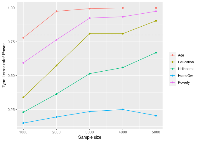
Here are examples of how to use other statistical inference models included in the package.
“Significant” is when the credible intervals don’t include zero. We access the 95% credible interval coverage with criterion “beta” and threshold 0.05.
bws_imod <- mpower::InferenceModel(model = "bws", iter = 2000, family = "gaussian", refresh = 0)
bws_power <- mpower::sim_power(xmod, ymod, bws_imod, s = 100, n = 1000,
                       cores=2, snr_iter=1000, errorhandling = "stop",
cluster_export = c("lm_demo"))Similar to BWS but is a frequentist method. The significance criterion is the p-value.
qgcomp_imod <- mpower::InferenceModel(model="qgc")
qg_power <- mpower::sim_power(xmod, ymod, qgcomp_imod, s = 100, n = 1000,
cores=2, snr_iter=1000, errorhandling = "remove")fin_imod <- InferenceModel(model="fin", nrun = 2000, verbose=F)
fin_power <- sim_power(xmod, ymod, fin_imod, s = 100, n = 1000,
cores=2, snr_iter=1000, errorhandling = "remove")bma_imod <- InferenceModel(model="bma", glm.family = "gaussian")
bma_power <- sim_power(xmod, ymod, bma_imod, s = 100, n = 1000,
cores=2, snr_iter=1000, errorhandling = "remove")bkmr_imod <- InferenceModel(model = "bkmr", iter = 5000, verbose = F)
bkmr_power <- sim_power(xmod, ymod, bkmr_imod, s = 100, n = 1000,
cores=2, snr_iter=1000, errorhandling = "remove")We show how to work with a binary outcome here. We load NHANES data from the 2015-2016 and 2017-2018 cycles included in our package and define a “true” outcome model that includes linear main effects and an interaction. We check the power to detect these effects using a logistic regression and a sample size of 2000 observations.
data("nhanes1518")
chems <- c("URXCNP", "URXCOP", "URXECP", "URXHIBP", "URXMBP", "URXMC1", "URXMCOH", "URXMEP",
"URXMHBP", "URXMHH", "URXMHNC", "URXMHP", "URXMIB", "URXMNP", "URXMOH", "URXMZP")
chems_mod <- mpower::MixtureModel(nhanes1518[, chems] %>% filter(complete.cases(.)),
                                  method = "resampling")
bmi_mod <- mpower::OutcomeModel(f = "0.2*URXCNP + 0.15*URXECP + 0.1*URXCOP*URXECP", family = "binomial")
logit_mod <- mpower::InferenceModel(model = "glm", family = "binomial")
logit_out <- mpower::sim_power(xmod=chems_mod, ymod=bmi_mod, imod=logit_mod,
                 s=100, n=2000, cores=2, snr_iter=5000)
logit_df <- summary(logit_out, crit="pval", thres=0.05, how="lesser")
#>
#> *** POWER ANALYSIS SUMMARY ***
#> Number of Monte Carlo simulations: 100
#> Number of observations in each simulation: 2000
#> Data generating process estimated SNR: 0.67
#> Inference model: glm
#> Significance criterion: pval
#>
#> Significance threshold: 0.05
#>
#> | | power|
#> |:-------|-----:|
#> |URXCNP | 0.18|
#> |URXCOP | 1.00|
#> |URXECP | 0.96|
#> |URXHIBP | 0.07|
#> |URXMBP | 0.03|
#> |URXMC1 | 0.05|
#> |URXMCOH | 0.05|
#> |URXMEP | 0.03|
#> |URXMHBP | 0.02|
#> |URXMHH | 0.05|
#> |URXMHNC | 0.05|
#> |URXMHP | 0.12|
#> |URXMIB | 0.02|
#> |URXMNP | 0.08|
#> |URXMOH | 0.07|
#> |URXMZP | 0.02|