Using
motoRneuron for motor unit synchronization
The purpose of this document is to get you started using the
motoRneuron package for analyzing motor unit data, even if
you’ve never used R before! So we will show you how to install the
toolbox through CRAN, access the functions, help files, and sample motor
unit data. Next, we will provide code to get typical time series data
into a workable format for our functions. Then we will go step-by-step
through some analyses with this sample data to demonstrate its
applicability.
Time-domain synchronization
It’s assumed that if you’re reading this, you have at least a grasp
of what motor unit synchronization means and what you hope to get out of
this package. Briefly, time-domain synchronization, in the neuromuscular
context we are presenting it, is the tendency of separate motor units
(i.e. motor neurons and their associated muscle fibers) to discharge
near-simultaneously (within 1 - 5 ms of each other) more often than
would be expected by chance. It is often interpreted as an indicator of
functional connectivity between motor neurons through common excitatory
post-synaptic potentials. This is quanitified by a cross correlation
analyses, which is essentially the core of this package. A peak in the
resulting cross correlation histogram represents a higher probability of
discharges at that latency. Indices that quantify the magnitude of the
peak are the primary outputs for the package.
Functions
recurrence_intervals() correlates the discharge times
of one motor unit against those of another motor unit.bin() creates a cross correlation histogram from the
recurrence intervals.plot_bins() plots the cross correlation histogram with
ggplot2.mu_synch() is an all-in-one function that automatically
performs the cross correlation process from steps 1 and 2 then assesses
the histogram for peaks using 3 optional methods (listed in 4). Six
commonly used synchronization indices are returned:
- Common Input Strength (CIS)
- k’
- k’-1
- E
- S
- Synch Index (SI)
- 3 methods of peak determination are available in
mu_synch() and as individual functions:
- Visual method -
visual_mu_synch()
- Cumulative Sum (Cumsum) method -
cumsum_mu_synch()
- Z-score method -
zscore_mu_synch()
Package Implementation
Install the package from the Comprehensive R Archive Network or
Github and attach it to your workspace with the following functions.
install.packages("motoRneuron")
install.pacakges("devtools")
devtools::install_github("tweedell/motoRneuron")
library(motoRneuron)
library(ggplot2)
View the package or any of the function help files by using ‘?’.
Data: motor_unit_data
Let’s load the sample motor unit data frame from the package into the
working environment and look at it before we perform any analyses with
it. The data is 30 seconds of 2 concurrently active motor units
discharging at semi-regular intervals. It was sampled at 1000 Hz.
motor_unit_data <- motoRneuron::motor_unit_data
head(motor_unit_data)
#>    Time motor_unit_1 motor_unit_2
#> 1 0.000            0            0
#> 2 0.001            0            0
#> 3 0.002            0            0
#> 4 0.003            0            0
#> 5 0.004            0            0
#> 6 0.005            0            0
You’ll see our first column is Time in seconds. The other columns
present the activation of “motor unit 1” and “motor unit 2” as a series
of binary values. A value of “1” indicates activation of the motor unit
at a specific time point, and a value of “0” indicates no activation.
Synchronization functions require actual discharge times as inputs… so
how is that obtained? We’ll help you out. We included this step because
this is a commonly used format for time series data like motor unit
discharges. To get the data in a usable form for our functions, we will
have to subset out only the time points for which each motor unit has a
value of 1.
motor_unit_1 <- data.frame(Time = motor_unit_data[["Time"]], MotorUnit1 = motor_unit_data[[2]])
motor_unit_1 <- subset(motor_unit_1, MotorUnit1 ==1)
motor_unit_1 <- as.vector(motor_unit_1$Time)
motor_unit_2 <- data.frame(Time = motor_unit_data[["Time"]], MotorUnit2 = motor_unit_data[[3]])
motor_unit_2 <- subset(motor_unit_2, MotorUnit2 ==1)
motor_unit_2 <- as.vector(motor_unit_2$Time)
You’ll see the individual motor unit data is now in vector format
containing only the time points of discharge for each motor unit.
head(motor_unit_1)
#> [1] 0.035 0.115 0.183 0.250 0.306 0.377
head(motor_unit_2)
#> [1] 0.100 0.205 0.298 0.377 0.471 0.577
So we’ve got our data in a format that our motoRneuron
functions will take.
Calculating
recurrence_intervals()
recurrence_intervals() calculates the recurrence
intervals based on how many recurrence interval orders is
specified (see image below). Specifically, they are calculated as the
timing difference between a discharge event in one (reference) motor
unit and the nearest forward and nearest backward discharge events in
another (event) motor unit. The motor unit used as the reference unit is
the unit with fewer discharges. Order refers to how many
discharges before and after we are including in our calculations.
Default settings are for first order recurrence intervals as previous
research has shown that false peaks are likely to appear with higher
orders. 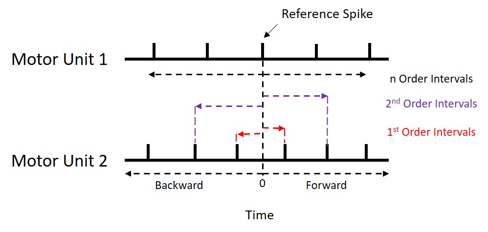
The function takes the vector arguments motor_unit_1 and motor_unit_2
containing activation times, along with an integer indicating the order.
The code below calculates the time differences between the reference
activation and the first and second forward and backward discharges from
the event motor unit.
recur <- recurrence_intervals(motor_unit_1, motor_unit_2, order = 2)
names(recur)
#>  [1] "Reference_Unit"                 "Number_of_Reference_Discharges"
#>  [3] "Reference_ISI"                  "Mean_Reference_ISI"
#>  [5] "Event_Unit"                     "Number_of_Event_Discharges"
#>  [7] "Event_ISI"                      "Mean_Event_ISI"
#>  [9] "Duration"                       "1"
#> [11] "2"
As you can see, various descriptors of the motor units are returned
as a list. For example, the mean inter-spike interval (ISI) for the
reference motor unit and the number of times the event motor unit
discharged are returned. At the end are vectors containing all the
recurrence intervals. In our example, with a recurrence interval order
of 2, the vectors produced are denoted “1” and “2”. The first pair of
numbers in vector [1] describes the recurrence interval time between the
first reference activation and the first order activation of the event
motor unit. The second pair of numbers indicates the recurrence interval
between the second reference activation and the corresponding first
order discharges from the event motor unit, and so on. For vector [2],
pairs of numbers describes the recurrence interval between the reference
discharge and the second order discharges from the event motor unit.
recur$'Reference_Unit'
#> [1] "motor_unit_2"
recur$Mean_Reference_ISI
#> [1] 0.098
recur$Number_of_Event_Discharges
#> [1] 443
head(recur$'1')
#> [1] -0.065  0.015 -0.022  0.045 -0.048  0.008
For demonstration purposes, we will only be using the first order
intervals.
Discretize recurrence
intervals with bin()
Only 2 arguments are needed for bin(); a vector
containing the recurrence intervals we just calculated and a numeric
indicating the bin size or width. Using unlist() will take
our intervals from our list format and convert them into a vector
format.
recur <- unlist(recur$`1`)
binned_data <- bin(recur, binwidth = 0.001)
A simple data frame is returned. Bin tells us how far
before or after the discharge of our reference motor unit that the other
motor unit discharged. Bin “0.000” represents the two motor units firing
at the exact same time. Freq is the frequency of that
interval occurring in the trial. Below we parse out from the data frame
only the bins representing +/- 0.015 s around the reference motor unit
discharge.
subset(binned_data, Bin >= -0.015 & Bin <= 0.015)
#>        Bin Freq
#> 87  -0.015    4
#> 88  -0.014    7
#> 89  -0.013   12
#> 90  -0.012    5
#> 91  -0.011    3
#> 92  -0.010    4
#> 93  -0.009    5
#> 94  -0.008   12
#> 95  -0.007   14
#> 96  -0.006    5
#> 97  -0.005   10
#> 98  -0.004   10
#> 99  -0.003    2
#> 100 -0.002   13
#> 101 -0.001    3
#> 102  0.000   21
#> 103  0.001   13
#> 104  0.002    1
#> 105  0.003    5
#> 106  0.004    4
#> 107  0.005    6
#> 108  0.006    4
#> 109  0.007    5
#> 110  0.008    7
#> 111  0.009    4
#> 112  0.010    4
#> 113  0.011    0
#> 114  0.012    9
#> 115  0.013    2
#> 116  0.014    4
#> 117  0.015    4
Visualization of
histogram with plot_bins()
plot_bins() leverages ggplot2 to graph the binned
recurrence intervals as a histogram. Mean bin size or average frequency
of the bins is indicated as a red line on the graph.
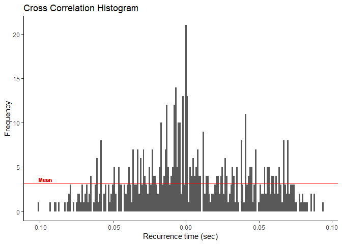 From
the graph, we can see that there are higher frequencies the nearer to
“0.000” we get. This may indicate that there is a more than likely
chance that these two motor units are functionally connected somehow. If
there is a peak in this histogram, then our synchronization functions
will determine where it is and calculate the various indices from
it.
From
the graph, we can see that there are higher frequencies the nearer to
“0.000” we get. This may indicate that there is a more than likely
chance that these two motor units are functionally connected somehow. If
there is a peak in this histogram, then our synchronization functions
will determine where it is and calculate the various indices from
it.
Synchronization functions
mu_synch() is the all-in-one function that calls both
recurrence_intervals() and bin() to perform
the initial analysis. It then uses the user-chosen methods for
determining if and where there is a peak. More specifically, it uses
these methods to find the upper and lower boundaries of a peak if there
is one. “Visual”, “Cumsum”, and “Zscore” methods are described below and
are available for peak determination. Alternatively, each method can be
called individually using their own functions.
synch_data <- mu_synch(motor_unit_1, motor_unit_2, method = c("Visual", "Cumsum", "Zscore"), order = 1, binwidth = 0.001, plot = F)
- Motor unit vectors, “order”, and “binwidth” are the same arguments
used for
recurrence_intervals() and
bin().
- “method” is a vector of character strings representing which methods
you want to call for peak boundary determination. Default is just
“Visual”.
mu_synch() calls each specified method by their
individual functions (described later).
- “plot” is a TRUE/FALSE logical on whether to output the histogram
from
plot_bins(). Default is FALSE.
A list is returned including the motor unit characteristic data and
the 6 synchronization indices (described below) for each of the methods
chosen.
## [1] "Data" "Visual Indices" "Zscore Indices" "Cumsum Indices"
synch_data$`Visual Indices`
## $`CIS`
## [1] 2.163168
##
## $kprime
## [1] 3.79096
##
## $kminus1
## [1] 2.79096
##
## $E
## [1] 0.2110322
##
## $S
## [1] 0.08638251
##
## $SI
## [1] 0.2117218
##
## $Peak.duration
## [1] 0.01
##
## $Peak.center
## [1] 0
synch_data$`Zscore Indices`
#> $CIS
#> [1] 1.714933
#>
#> $kprime
#> [1] 4.284502
#>
#> $kminus1
#> [1] 3.284502
#>
#> $E
#> [1] 0.1673037
#>
#> $S
#> [1] 0.06848299
#>
#> $SI
#> [1] 0.1678505
#>
#> $Peak.duration
#> [1] NA
#>
#> $Peak.center
#> [1] NA
synch_data$`Cumsum Indices`
#> $CIS
#> [1] 2.163168
#>
#> $kprime
#> [1] 3.79096
#>
#> $kminus1
#> [1] 2.79096
#>
#> $E
#> [1] 0.2110322
#>
#> $S
#> [1] 0.08638251
#>
#> $SI
#> [1] 0.2117218
#>
#> $Peak.duration
#> [1] 0.01
#>
#> $Peak.center
#> [1] 0
- Common Input Strength (CIS) = extra counts in peak / duration of
time both motor units are active (s)
- k’ = total counts in peak / expected counts in peak
- k’-1 = extra counts in peak / expected counts in peak
- E = extra counts in peak / number of reference discharges
- S = extra counts in peak / (number of reference discharges + number
of event discharges))
- Synch Index (SI) = (extra counts in peak / (total counts in peak /
2))
Expected counts are the number of counts within the peak boundaries
that we would expect to have if the two motor units were independent.
This is usually calculated as the mean bin count of the baseline portion
of the histogram (<= -0.06 s and >= 0.06 s). This is explained
more in depth in the determination methods sections.
Peak location is also returned with the Synchronization Indices:
- Peak center - Describes the location of the middle of the peak and
is calculated as the median between the upper and lower boundaries.
- Peak Duration - Describes the broadness of the peak and is
calculated as the range for the upper and lower boundaries.
Visual Determination
Visual determination of peaks in a cross correlation histogram takes
a more subjective approach than other automated detection algorithms.
Investigators are usually asked where they see peaks, but as bin count
or bin frequency can vary greatly, discerning areas of greater frequncy
can be difficult for the human eye. To make it easier, the mean baseline
bin frequency (considered the mean frequncy of bins >= -0.06 s and
<= 0.06 s) is subtracted from each bin. Then the cumulative sum is
taken from these normlized bins. This method allows for normally
difficult to see increases in frequency (or peaks) to show up as
deflections in the graph. The boundaries of these deflections are the
boundaries of the peak. When called, this function automatically
configures the normalized cumulative sum then leverages the dygraphs
package to interactively display it for the user to view and determine
peak boundaries.
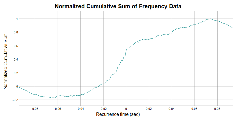
In the graph above you see the x-axis is just like the bins of the
cross correlation histogram, representing the time difference between
firings of the motor units. The y-axis notes the normalized cumulative
sum values for each bin. The mouse can be used to drag a vertical cursor
along the graph. This will display x and y values.
When the function is called, the user is prompted in the console to
indicate whether they actually see a deflection in the graph near time
“0.00” that may indicate a peak (y/n).
Is there a discernable change in slope or deflection near time 0 (y/n)?
- If no, default bins of +/- 0.005 s are chosen and fed into the
calculations.
- If yes, the user is prompted one at a time to input the left and
right boundaries (time points in seconds) of a peak seen as a dramatic
slope increase in the cumulative sum graph around 0. These peak boundary
bins are then fed into the calculations.
Enter the time (in sec) of the start of slope change (left or lower boundary of peak) of the graph:
Enter the time (in sec) of the end of slope change (right or upper boundary of peak) of the graph:
The synchronization function for visual determination is below. A
list similar to mu_synch() is returned.
visual_mu_synch(motor_unit_1, motor_unit_2, order = 1, binwidth = 0.001, get_data = T, plot = F)
Cumsum Determination
The cumulative sum method is an automated method that does not
require input by the user. Peak boundaries are determined as the bins
associated with 10% and 90% of the range (maximum minus minimum) of the
cumulative sum. The peak is considered significant if its mean bin count
exceeds the sum of the mean and 1.96 * standard deviation of the
baseline bins (<= -0.06 s and >= 0.06 s). If no significant peak
is detected, a default +/- 0.005 s peak duration is used.
cumsum_mu_synch(motor_unit_1, motor_unit_2, order = 1, binwidth = 0.001, get_data = T, plot = F)
Z-score Determination
Another automated method for peak determination is the z-score
method, which relies on the assumption that if two motor units are
independent (i.e. no synchronization) then the cross correlation between
them is random and the histogram would appear flat. So first, a random
uniform distribution is used to produce a flat histogram and calculate a
mean + 1.96 * standard deviation threshold for the experimental cross
correlation histogram. Any bins in the experimental histogram within +/-
0.01 s of 0.000 that crosses the threshold are considered to be
significantly greater than expected due to chance and subsequently used
for analysis. If no peaks are detected, synchronization indices of 0 are
returned. Because the z-score method tests each bin individually,
peak bins are not necessarily adjacent. Therefore, peak duration
and peak center are returned as NA.
zscore_mu_synch(motor_unit_1, motor_unit_2, order = 1, binwidth = 0.001, get_data = T, plot = F)