meltt provides a method for integrating event data in R.
Event data seeks to capture micro-level information on event occurrences
that are temporally and spatially disaggregated. For example,
information on neighborhood crime, car accidents, terrorism events, and
marathon running times are all forms of event data. These data provide a
highly granular picture of the spatial and temporal distribution of a
specific phenomena.
In many cases, more than one event dataset exists capturing related topics – such as, one dataset that captures information on burglaries and muggings in a city and another that records assaults – and it can be useful to combine these data to bolster coverage, capture a broader spectrum of activity, or validate the coding of these datasets. However, matching event data is notoriously difficult:
Jittering Locations, different geo-referencing software can produce slightly different longitude and latitude locations for the same place. This results in an artificial geo-spatial “jitter” around the same location.
Temporal Fuzziness, given how information about events are collected, the exact date of an event reported might differ from source to source. For example, if data is generated using news reports, they might differ in their reporting of the exact timing of the event—especially if precise on-the-ground information is hard to come by. This creates a temporal fuzziness where the same empirical event falls on different days in different datasets .
Conceptual Differences, different event datasets are built for different reasons, meaning each dataset will likely contain its own coding schema for the same general category. For example, a dataset recording local muggings and burglaries might have a schema that records these types of events categorically (i.e “mugging”, “break in”, etc.), whereas another crime dataset might record violent crimes and do so ordinally (1, 2, 3, etc.). Both datasets might be capturing the same event (say, a violent mugging) but each has its own method of coding that event.
In the past, to overcome these hurdles, researchers have typically
relied on hand-coding to systematically match these data, which needless
to say, is extremely time consuming, error-prone, and hard to reproduce.
meltt provides a way around this problem by implementing a
method that automates the matching of different event datasets in a
fast, transparent, and reproducible way.
More information about the specifics of the method can also be found in our article in the Journal of Conflict Resolution as well as in the package documentation.
The package can be installed through the CRAN repository.
install.packages("meltt")Or the development version from Github
# install.packages("devtools")
devtools::install_github("kdonnay/meltt")
The package requires that users have Python (>= 3.6) installed on
their computer. To quickly get Python, install an Anaconda
platform. meltt will use the program in the background.
In the following illustrations, we use (simulated) Maryland car crash data. These data constitute three separate data sets capturing the same thing: car crashes in the state of Maryland for January 2012. But each data set differs in how it codes information on the car’s color, make, and the type of accident.
data("crashMD")str(crash_data1)## 'data.frame': 71 obs. of 9 variables:
## $ dataset : chr "crash_data1" "crash_data1" "crash_data1" "crash_data1" ...
## $ event : int 1 2 3 4 5 6 7 8 9 10 ...
## $ date : Date, format: "2012-01-01" "2012-01-01" ...
## $ enddate : Date, format: "2012-01-01" "2012-01-02" ...
## $ latitude : num 39.1 38.6 39.1 38.3 38.3 ...
## $ longitude : num -76 -75.7 -76.9 -75.6 -76.5 ...
## $ model_tax : chr "Full-Sized Pick-Up Truck" "Mid-Size Car" "Cargo Van" "Mini Suv" ...
## $ color_tax : chr "210-180-140" "173-216-230" "210-180-140" "139-137-137" ...
## $ damage_tax: chr "1" "5" "4" "4" ...str(crash_data2)## 'data.frame': 64 obs. of 9 variables:
## $ dataset : chr "crash_data2" "crash_data2" "crash_data2" "crash_data2" ...
## $ event : int 1 2 3 4 5 6 7 8 9 10 ...
## $ date : Date, format: "2012-01-01" "2012-01-01" ...
## $ enddate : Date, format: "2012-01-01" "2012-01-01" ...
## $ latitude : num 39.1 39.1 39.1 39 38.5 ...
## $ longitude : num -76.9 -76 -76.7 -76.2 -76.6 ...
## $ model_tax : chr "Van" "Pick-Up" "Small Car" "Large Family Car" ...
## $ color_tax : chr "#D2b48c" "#D2b48c" "#D2b48c" "#Ffffff" ...
## $ damage_tax: chr "Flip" "Mid-Rear Damage" "Front Damage" "Front Damage" ...str(crash_data3)## 'data.frame': 60 obs. of 9 variables:
## $ dataset : chr "crash_data3" "crash_data3" "crash_data3" "crash_data3" ...
## $ event : int 1 2 3 4 5 6 7 8 9 10 ...
## $ date : Date, format: "2012-01-01" "2012-01-01" ...
## $ enddate : Date, format: "2012-01-01" "2012-01-01" ...
## $ latitude : num 39.1 39.1 38.4 39.1 38.6 ...
## $ longitude : num -76.9 -76 -75.4 -76.6 -76 ...
## $ model_tax : chr "Cargo Van" "Standard Pick-Up" "Mid-Sized" "Small Sport Utility Vehicle" ...
## $ color_tax : chr "Light Brown" "Light Brown" "Gunmetal" "Red" ...
## $ damage_tax: chr "Vehicle Rollover" "Rear-End Collision" "Sideswipe Collision" "Vehicle Rollover" ...Each dataset contain variables that code:
date: when the event occurred;enddate: if the event occurred across more than one
day, i.e. an “episode”;longitude & latitude: geo-location
information;model_tax: coding scheme of the type of car;color_tax: coding scheme of the color of the car;damage_tax: coding scheme of the type of accident.The variable names across dataset have already been standardized (for reasons further outlined below).
The goal is to match these three event datasets to locate which
reported events are the same, i.e., the corresponding data set entries
are duplicates, and which are unique. meltt formalizes all
input assumptions the user needs to make in order to match these
data.
First, the user has to specify a spatial and temporal window that any potential match could plausibly fall within. Put differently, how close in space and time does an event need to be to qualify as potentially reporting on the same incident?
Second, to articulate how different coding schemes overlap, the user needs to input an event taxonomy. A taxonomy is a formalization of how variables overlap, moving from as granular as possible to as general as possible. In this case, it describes how the coding of the three car-specific properties (model, color, damage) across our three data sets correspond.
Among the three variables that exist in all three in datasets we
consider the damage_tax variable recorded in each of
dataset for an in-depth example:
unique(crash_data1$damage_tax)## [1] "1" "5" "4" "6" "2" "3" "7"unique(crash_data2$damage_tax)## [1] "Flip" "Mid-Rear Damage"
## [3] "Front Damage" "Side Damage While In Motion"
## [5] "Hit Tree" "Side Damage"
## [7] "Hit Property"unique(crash_data3$damage_tax)## [1] "Vehicle Rollover" "Rear-End Collision"
## [3] "Sideswipe Collision" "Object Collisions"
## [5] "Side-Impact Collision" "Liable Object Collisions"
## [7] "Head-On Collision"Each variable records information on the type of accident a little differently. The idea of introducing a taxonomy is then, as mentioned before, to generalize across each category by clarifying how each coding scheme maps onto the other.
str(crash_taxonomies$damage_tax)## 'data.frame': 21 obs. of 3 variables:
## $ data.source : chr "crash_data1" "crash_data1" "crash_data1" "crash_data1" ...
## $ base.categories: chr "1" "2" "3" "4" ...
## $ damage_level1 : chr "Multi-Vehicle Accidents" "Multi-Vehicle Accidents" "Multi-Vehicle Accidents" "Single Car Accidents" ...The crash_taxonomies object contains three pre-made
taxonomies for each of the three overlapping variable categories. As you
can see, the damage_tax contains only a single level
describing how the different coding schemes overlap. When matching the
data, meltt uses this information to score potential
matches that are proximate in space and time.
Likewise, we similarly formalized how the model_tax and
color_tax variables map onto one another.
str(crash_taxonomies$color_tax)## 'data.frame': 39 obs. of 4 variables:
## $ data.source : chr "crash_data1" "crash_data1" "crash_data1" "crash_data1" ...
## $ base.categories: chr "255-0-0" "0-0-128" "255-255-255" "0-100-0" ...
## $ col_level1 : chr "Red Shade" "Blue Shade" "Greyscale Shade" "Green Shade" ...
## $ col_level2 : chr "Dark" "Dark" "Light" "Dark" ...str(crash_taxonomies$model_tax)## 'data.frame': 31 obs. of 5 variables:
## $ data.source : chr "crash_data1" "crash_data1" "crash_data1" "crash_data1" ...
## $ base.categories: chr "Economy Car" "Mid-Sized Luxery Car" "Small Family Car" "Mpv" ...
## $ make_level1 : chr "B-Segment Small Cars" "E-Segment Executive Cars" "C-Segment Medium Cars" "M-Segment Multipurpose Cars" ...
## $ make_level2 : chr "Passenger Car" "Passenger Car" "Passenger Car" "Mpv" ...
## $ make_level3 : chr "Small Vehicle" "Small Vehicle" "Small Vehicle" "Large Vehicle" ...The color and model taxonomies contain more levels than the damage
taxonomy representing specific to increasingly broader categories under
which both color and model of the cars can be described. For example,
the model_tax goes from make_level1, which
contains a schema with 7 unique entries using the Euro coding of car
models as a way of specifying overlap, to make_level3,
which contains a schema with only two categories (i.e. differentiation
between large and small vehicles).
Generally, specifications of taxonomy levels can be as granular or as broad as one chooses. The more fine-grained the levels one includes to describe the overlap, the more specific the match. At the same time, if categories are too narrow, it is difficult to conceptualize potential matches across datasets. As a rule, there is thus a trade off between specific categories that can better differentiate among possible duplicate entries and unspecific categories that more easily recognize potentially matching information across datasets.
As a general rule, we therefore recommend to include, whenever it is
conceptually warranted, both specific fine-grained categories and a few
increasingly broader ones. In this case, meltt will have
more information to work with when differentiating between sets of
potential matches. In establishing which entries are most likely to
correspond, meltt in case of more than two potential
matches in one dataset always automatically favors the one that more
precisely corresponds. A good taxonomy is the key to matching
data, and is the primary vehicle by which a user’s assumptions –
regarding how data fits together – is made transparent.
A few technical things to note:
data.frame is read into meltt as a
single list object.str(crash_taxonomies)
# List of 3
# $ model_tax :'data.frame': 31 obs. of 5 variables:
# ..$ data.source : chr [1:31] "crash_data1" "crash_data1" "crash_data1" "crash_data1" ...
# ..$ base.categories: chr [1:31] "Economy Car" "Mid-Sized Luxery Car" "Small Family Car" "Mpv" ...
# ..$ make_level1 : chr [1:31] "B-Segment Small Cars" "E-Segment Executive Cars" "C-Segment Medium Cars" "M-Segment Multipurpose Cars" ...
# ..$ make_level2 : chr [1:31] "Passenger Car" "Passenger Car" "Passenger Car" "Mpv" ...
# ..$ make_level3 : chr [1:31] "Small Vehicle" "Small Vehicle" "Small Vehicle" "Large Vehicle" ...
# $ color_tax :'data.frame': 39 obs. of 4 variables:
# ..$ data.source : chr [1:39] "crash_data1" "crash_data1" "crash_data1" "crash_data1" ...
# ..$ base.categories: chr [1:39] "255-0-0" "0-0-128" "255-255-255" "0-100-0" ...
# ..$ col_level1 : chr [1:39] "Red Shade" "Blue Shade" "Greyscale Shade" "Green Shade" ...
# ..$ col_level2 : chr [1:39] "Dark" "Dark" "Light" "Dark" ...
# $ damage_tax:'data.frame': 21 obs. of 3 variables:
# ..$ data.source : chr [1:21] "crash_data1" "crash_data1" "crash_data1" "crash_data1" ...
# ..$ base.categories: chr [1:21] "1" "2" "3" "4" ...
# ..$ damage_level1 : chr [1:21] "Multi-Vehicle Accidents" "Multi-Vehicle Accidents" "Multi-Vehicle Accidents" "Single Car Accidents" ...meltt relies on simple naming
conventions to identify which variable is what when matching.names(crash_taxonomies)
# [1] "model_tax" "color_tax" "damage_tax"
colnames(crash_data1)[7:9]
# [1] "model_tax" "color_tax" "damage_tax"
colnames(crash_data2)[7:9]
# [1] "model_tax" "color_tax" "damage_tax"
colnames(crash_data3)[7:9]
# [1] "model_tax" "color_tax" "damage_tax"Each taxonomy must contain a data.source and
base.categories column: this last convention helps
meltt identify which variable is contained in which data
object. The data.source column should reflect the
names of the of the data objects for input
data and the base.categories should reflect
the original coding of the variable on which the taxonomy is
built.
Each input dataset must contain a
date,enddate (if one exists),
longitude, and latitude column: the
variables must be named accordingly (no deviations in naming
conventions). The dates should be in an R date format
(as.Date()), and the geo-reference information must be
numeric (as.numeric()).
Once the taxonomy is formalized, matching several datasets is
straightforward. The meltt() function takes four main
arguments: - ...: input data; - taxonomies =:
list object containing the user-input taxonomies; -
spatwindow =: the spatial window (in kilometers); -
twindow =: the temporal window (in days).
Below we assume that any two events in two different datasets occurring within 4 kilometers and 2 days of each other could plausibly be the same event. This ‘’fuzziness’’ basically sets the boundaries on how precise we believe the spatial location and timing of events is coded. It is usually best practice to vary these specifications systematically to ensure that no one specific combination drives the outcomes of the integration task.
We then assume that event categories map onto each other according to
the way that we formalized in the taxonomies outlined above. We fold all
this information together using the meltt() function and
then store the results in an object named output.
output <- meltt(crash_data1, crash_data2, crash_data3,
                taxonomies = crash_taxonomies,
                spatwindow = 4,
                twindow = 2)
meltt also contains a range of adjustments to offer the
user additional controls regarding how the events are matched. These
auxiliary arguments are: - smartmatch: when
TRUE (default), all available taxonomy levels are used and
meltt uses a matching score that ensures that fine-grained
agreements is favored over broader agreement, if more than one taxonomy
level exists. When FALSE, only specific taxonomy levels are
considered. - certainty: specification of the the exact
taxonomy level to match on when smartmatch = FALSE. -
partial: specifies whether matches along only some of the
taxonomy dimensions are permitted. - averaging: implement
averaging of all values events are match on when matching across
multiple data.frames. That is, as events are matched dataset by dataset,
the metadata is averaged. (Note: that this can generate distortion in
the output). - weight: specified weights for each taxonomy
level to increase or decrease the importance of each taxonomy’s
contribution to the matching score.
At times, one might want to know which taxonomy level is doing the
heavy lifting. By turning off smartmatch, and specifying
certain taxonomy levels by which to compare events, or by weighting
taxonomy levels differently, one is able to better assess which
assumptions are driving the final integration results. This can help
with fine-tuning the input assumptions for meltt to gain
the most valid match possible.
When printed, the meltt object offers a brief summary of
the output.
output## MELTT Complete: 3 datasets successfully integrated.
## =========================================================
## Total No. of Input Observations: 195
## No. of Unique Obs (after deduplication): 140
## No. of Unique Matches: 34
## No. of Duplicates Removed: 55
## =========================================================In matching the three car crash datasets, there are 195 total entries
(i.e. 71 entries from crash_data1, 64 entries from
crash_data2, and 60 entries from crash_data3).
Of those 195, 140 of them are unique – that is, no entry from another
dataset matched up with them. 55 entries, however, were found to be
duplicates identified within 34 unique matches.
The summary() function offers a more informed summary of
the output.
summary(output)##
## MELTT output
## ============================================================
## No. of Input Datasets: 3
## Data Object Names: crash_data1, crash_data2, crash_data3
## Spatial Window: 4km
## Temporal Window: 2 Day(s)
##
## No. of Taxonomies: 3
## Taxonomy Names: model_tax, color_tax, damage_tax
## Taxonomy Depths: 3, 2, 1
##
## Total No. of Input Observations: 195
## No. of Unique Matches: 34
## - No. of Event-to-Event Matches: 26
## - No. of Episode-to-Episode Matches: 8
## No. of Duplicates Removed: 55
## No. of Unique Obs (after deduplication): 140
## ------------------------------------------------------------
## Summary of Overlap
## crash_data1 crash_data2 crash_data3 Freq
## X 41
## X 34
## X 31
## X X 5
## X X 4
## X X 4
## X X X 21
## ============================================================
## *Note: 6 episode(s) flagged as potentially matching to an event.
## Review flagged match with meltt.inspect()Given that meltt objects can be saved and referenced later, the summary function offers a recap on the input parameters and assumptions that underpin the match (i.e. the datasets, the spatiotemporal window, the taxonomies, etc.). Again, information regarding the total number of observations, the number of unique and duplicate entries, and the number matches found is reported, but this time information regarding how many of those matches were event-to-event (i.e. events that played out along one time unit where the date is equal to the end date) and episode-to-episode (i.e. events that played out over a couple of days).
NOTE: Events that have been flagged as matching to episodes require manual review using the
meltt.inspect()function. The summary output tells us that 6 episodes are flagged as potentially matching. Technically speaking, episodes (events with different start and end dates) and events are at different units of analysis; thus, user discretion is required to help sort out these types of matches. Themeltt.inspect()function eases this process of manual assessment. We are developing a shiny app to help assessment further in this regard.
A summary of overlap is also provided, articulating how the different input datasets overlap and where. For example, of the 34 matches 5 occurred between crash_data1 and crash_data2, 4 between crash_data1 and crash_data3, 4 between crash_data2 and crash_data3, and 21 between all three.
For quick visualizations of the matched output, meltt
contains three plotting functions.
plot() offers a bar plot that graphically articulates
the unique and overlapping entries. Note that the entries from the
leading dataset (i.e. the dataset first entered into meltt) is all
black. In this representation, all matching (or duplicate) entries are
expressed in reference to the datasets that came before it. Any match
found in crash_data2 is with respect to crash_data1, any in crash_data3
with respect to crash_data1 and crash_data2. All the plotting function
are written using ggplot2 so they can be stored in an
object and altered accordingly.
plot(output)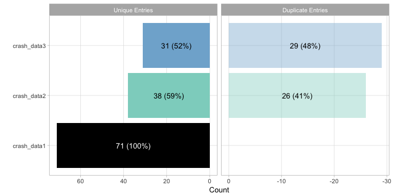
tplot() offers a time series plot of the meltt output.
The plot works as a reflection, where raw counts of the unique entries
are plotted right-side up and the raw counts of the removed duplicates
are plotted below it. This offers a quick snapshot of when
duplicates are found. Temporal clustering of duplicates may indicate an
issue with the data and/or the input assumptions, or it’s potentially
evidence of a unique artifact of the data itself.
Users can specify the temporal unit that the data should be binned (day, week, month, year).
t1 <- tplot(output, time_unit="days")
t2 <- tplot(output, time_unit="weeks")
gridExtra::grid.arrange(t1,t2)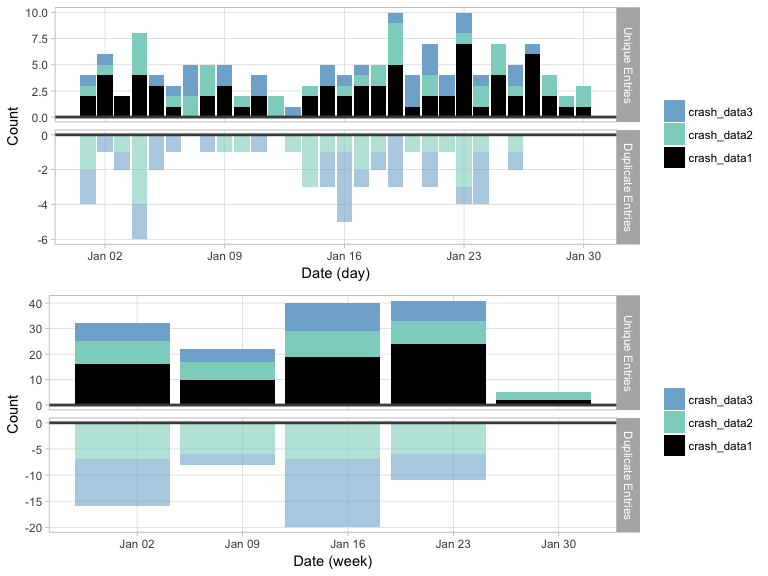
Similarly, mplot() presents an interactive summary of
the spatial distribution of the data by plotting the spatial points
using leaflet. The goal is to get a sense of the spatial
distribution of the matches to both identify any
clustering/disproportionate coverage in the areas that matches are
located, and to also get a sense of the spread of the integrated output.
Building the function around leaflet allows for easy
interactive exploration from within an R notebook or viewer.
To view unique and matched events (i.e. the types of data retrieved
via meltt_data()):
mplot(output) 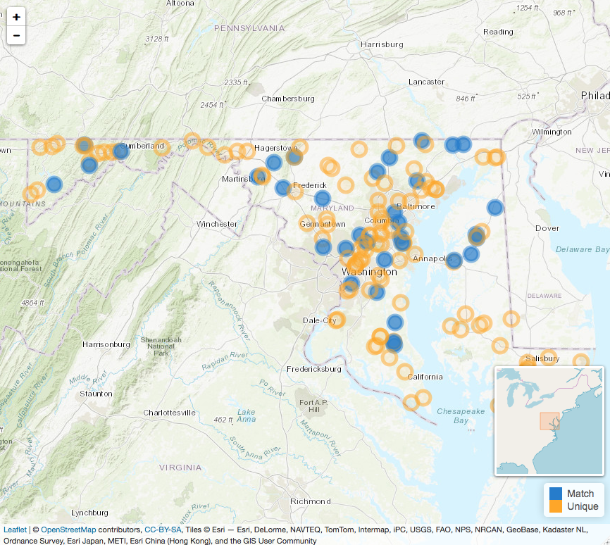
To view duplicate and matched events (i.e. the types of data
retrieved via meltt_duplicates()), set the
matching= argument to TRUE.
mplot(output, matching = TRUE) meltt provides two methods for extracting data from the
output object.
meltt_data() returns the de-duplicated data along with
any necessary columns the user might need. This is the primary function
for extracting matched data and moving on with subsequent analysis. The
columns = argument takes any vector of variable names and
returns those variables in the output. If no variables are specified,
meltt returns the spatio-temporal and taxonomy variables
that were employed during the match. In addition, the function returns a
unique event and data ID for reference.
uevents <- meltt_data(output, columns = c("date","model_tax"))

str(uevents)
## 'data.frame': 140 obs. of 6 variables:
## $ dataset : chr "crash_data1" "crash_data1" "crash_data2" "crash_data3" ...
## $ event : int 1 2 3 3 3 4 5 6 4 5 ...
## $ date : Date, format: "2012-01-01" "2012-01-01" ...
## $ latitude : num 39.1 38.6 39.1 38.4 39.1 ...
## $ longitude: num -76 -75.7 -76.7 -75.4 -76.9 ...
## $ model_tax: chr "Full-Sized Pick-Up Truck" "Mid-Size Car" "Small Car" "Mid-Sized" ...meltt_duplicates(), on the other hand, returns a data
frame of all events that matched up. This provides a quick way of
examining and assessing the events that matched. Since the quality of
any match is only as good as the assumptions we input, its key that the
user qualitatively evaluate the meltt output to assess whether any
assumptions should be adjusted. Like meltt_data(), the
columns = argument can be customized to return variables of
interest.
Note that the data is presented differently than in
meltt_data(); here each dataset (and its corresponding
variables) is presented in a separate column. This representation is
chose for ease of comparison. For example, the entry for row 1 denotes
that the 55th entry in the crash_data2 data matched with entry 57 from
the crash_data3, whereas no entry from crash_data1 matched (as indicated
with “dataID” and “eventID” 0 and “date” NA). The requested columns are
intended to assist with validation.
dups <- meltt_duplicates(output, columns = c("date"))
str(dups)
## 'data.frame': 34 obs. of 9 variables:
## $ crash_data1_dataID : num 0 0 0 0 1 1 1 1 1 1 ...
## $ crash_data1_eventID: num 0 0 0 0 1 3 7 9 10 12 ...
## $ crash_data2_dataID : num 2 2 2 2 2 2 0 2 2 2 ...
## $ crash_data2_eventID: num 55 8 39 44 2 1 0 5 7 10 ...
## $ crash_data3_dataID : num 3 3 3 3 3 3 3 3 3 3 ...
## $ crash_data3_eventID: num 57 10 36 44 2 1 4 8 7 6 ...
## $ crash_data3_date : Date, format: "2012-01-26" "2012-01-05" ...
## $ crash_data2_date : Date, format: "2012-01-25" "2012-01-04" ...
## $ crash_data1_date : Date, format: NA NA ...meltt also offers users a way of validating the quality
of any integration task with the function meltt_validate().
The function proceeds in three steps:
meltt_validate() allows users to randomly sample a
proportion of matching pairs and then generates a “control group” of two
entries that are close to the matching entries but were not identified
as matches. This sampled subset of the data is then assessed manually by
the user in step 2.meltt_validate() collapses
into a simple print function that reports accuracy diagnostics (i.e. the
true/false positive/negative rates).meltt_validate(output, sample_prop = .5, description.vars = c("date","model_tax"))Given that meltt operates primarily on user input
assumptions, validating the output of any integration task is key as
assumptions often need to be adjusted to optimize the matching
algorithm.
Like most S3 objects, the output from meltt is a nested
list containing a range of useful information. The output from
meltt retains the original input data and taxonomies and
the specification assumptions as well as lists of contender events
(i.e. events that were flagged as potential matches but did not match as
closely as another event). Note that we are expanding meltt’s
functionality to include more posterior function to ease extraction of
this information, but for now, it can simply be accessed using the usual
$ key convention.
names(output)## [1] "processed" "inputData" "parameters" "inputDataNames"
## [5] "taxonomy"str(output$processed$event_contenders)## 'data.frame': 41 obs. of 12 variables:
## $ dataset : num 1 1 1 1 1 1 1 1 1 1 ...
## $ event : num 1 3 9 10 12 13 19 26 27 30 ...
## $ bestmatch_data : num 2 2 2 2 2 2 2 2 2 2 ...
## $ bestmatch_event: num 2 1 5 7 10 6 21 25 26 31 ...
## $ bestmatch_score: num 0 0 0 0 0 0 0 0 0 0 ...
## $ runnerUp1_data : num 0 0 2 0 0 0 0 0 0 0 ...
## $ runnerUp1_event: num 0 0 2 0 0 0 0 0 0 0 ...
## $ runnerUp1_score: num 0 0 0.5 0 0 0 0 0 0 0 ...
## $ runnerUp2_data : num 0 0 0 0 0 0 0 0 0 0 ...
## $ runnerUp2_event: num 0 0 0 0 0 0 0 0 0 0 ...
## $ runnerUp2_score: num 0 0 0 0 0 0 0 0 0 0 ...
## $ events_matched : num 1 1 2 1 1 1 1 1 1 1 ...meltt in R using
citation(package = 'meltt')