![]()
![]()
![]()
Package: markovmix
0.1.3
Author: Xiurui Zhu
Modified: 2023-05-26 19:42:22
Compiled: 2023-12-02 18:34:35
The goal of markovmix is to fit mixture of Markov chains
of higher orders from multiple sequences. It is also compatible with
ordinary 1-component, 1-order or single-sequence Markov chains. Various
utility functions are provided to derive transition patterns, transition
probabilities per component and component priors. In addition,
print(), predict() and component
extracting/replacing methods are also defined as a convention of mixture
models.
You can install the released version of markovmix from
CRAN with:
install.packages("markovmix")Alternatively, you can install the developmental version of
markovmix from github
with:
remotes::install_github("zhuxr11/markovmix")Before start, we generate some sequences with a finite set of states, just as those to fit a Markov chain.
library(markovmix)library(purrr)
#>
#> Attaching package: 'purrr'
#> The following object is masked from 'package:testthat':
#>
#> is_null
# Define Markov states
mk_states <- LETTERS[seq_len(4L)]
# Define number of sequences
mk_size <- 100L
# Define sequence length range
mk_len_range <- seq_len(10L)
# Define a helper function to generate sequence list
gen_seq_list <- function(size, len_range, states, seed = NULL) {
if (is.null(seed) == FALSE) {
set.seed(seed)
}
purrr::map(seq_len(size), ~ sample(states, sample(len_range, 1L), replace = TRUE))
}
mk_seq_list <- gen_seq_list(size = mk_size, len_range = mk_len_range, states = mk_states, seed = 1111L)
head(mk_seq_list)
#> [[1]]
#> [1] "B" "B" "D" "A" "B" "B"
#>
#> [[2]]
#> [1] "C" "C" "D" "C" "C" "A" "A" "B" "D" "B"
#>
#> [[3]]
#> [1] "C" "A"
#>
#> [[4]]
#> [1] "A"
#>
#> [[5]]
#> [1] "A" "D" "B" "B"
#>
#> [[6]]
#> [1] "A" "B"First, we fit a 1-order Markov chain, the most commonly used type.
mk_fit <- fit_markov_mix(seq_list = mk_seq_list, states = mk_states)
#> Fitting Markov chain with a single (non-mixture) component ...
print(mk_fit)
#> This is a 1-order Markov chain.
#> Transition matrix:
#>           A         B         C         D
#> A 0.2149533 0.2616822 0.2803738 0.2429907
#> B 0.2200000 0.2400000 0.2500000 0.2900000
#> C 0.2232143 0.2232143 0.2142857 0.3392857
#> D 0.2803030 0.2272727 0.2196970 0.2727273
Then, we fit a 2-order Markov chain.
mk_fit2 <- fit_markov_mix(seq_list = mk_seq_list, order. = 2L, states = mk_states)
#> Fitting Markov chain with a single (non-mixture) component ...
print(mk_fit2)
#> This is a 2-order Markov chain.
#> Transition matrix:
#>               A         B          C         D
#> A->A 0.15000000 0.3500000 0.20000000 0.3000000
#> A->B 0.15000000 0.2000000 0.25000000 0.4000000
#> A->C 0.36000000 0.2000000 0.16000000 0.2800000
#> A->D 0.20000000 0.2500000 0.25000000 0.3000000
#> B->A 0.31250000 0.1250000 0.31250000 0.2500000
#> B->B 0.23529412 0.4117647 0.05882353 0.2941176
#> B->C 0.23809524 0.2380952 0.23809524 0.2857143
#> B->D 0.39285714 0.1785714 0.28571429 0.1428571
#> C->A 0.20000000 0.2000000 0.30000000 0.3000000
#> C->B 0.29411765 0.1764706 0.35294118 0.1764706
#> C->C 0.18181818 0.2727273 0.18181818 0.3636364
#> C->D 0.27586207 0.1034483 0.34482759 0.2758621
#> D->A 0.25000000 0.2187500 0.37500000 0.1562500
#> D->B 0.25000000 0.2083333 0.25000000 0.2916667
#> D->C 0.08695652 0.2608696 0.26086957 0.3913043
#> D->D 0.21428571 0.3214286 0.07142857 0.3928571
Finally, we fit a 3-component mixture of 2-order Markov chains, with randomly generated soft clustering probabilities for each sequence.
# Define number of components
mk_n_comp <- 3L
set.seed(2222L)
mk_clusters <- matrix(runif(length(mk_seq_list) * mk_n_comp), nrow = length(mk_seq_list), ncol = mk_n_comp)
mk_mix_fit2 <- fit_markov_mix(seq_list = mk_seq_list, order. = 2L, states = mk_states, clusters = mk_clusters)
print(mk_mix_fit2)
#> This is a 3-component mixture of 2-order Markov chains.
#>
#> Component 1: prior = 0.312888
#> Transition matrix:
#>              A         B          C         D
#> A->A 0.1169575 0.3560494 0.26867335 0.2583198
#> A->B 0.1801687 0.2006756 0.26776742 0.3513882
#> A->C 0.3175922 0.1573649 0.23078407 0.2942588
#> A->D 0.1358512 0.2751465 0.24779010 0.3412122
#> B->A 0.4378156 0.1175067 0.29539207 0.1492856
#> B->B 0.2220438 0.4673616 0.06273356 0.2478610
#> B->C 0.2186025 0.2576454 0.18613038 0.3376218
#> B->D 0.3619600 0.1604362 0.30587425 0.1717296
#> C->A 0.2081094 0.2091141 0.26581457 0.3169619
#> C->B 0.2241448 0.2723052 0.37160938 0.1319407
#> C->C 0.1396863 0.3332129 0.10758567 0.4195152
#> C->D 0.2879243 0.1244539 0.33908336 0.2485385
#> D->A 0.2244122 0.2455392 0.35763150 0.1724172
#> D->B 0.1870143 0.3054860 0.19841956 0.3090801
#> D->C 0.1713767 0.3194105 0.14752264 0.3616902
#> D->D 0.2345398 0.3229447 0.04483108 0.3976844
#>
#> Component 2: prior = 0.3381894
#> Transition matrix:
#>               A          B          C         D
#> A->A 0.12849557 0.28940102 0.20291519 0.3791882
#> A->B 0.14949616 0.15719777 0.24873975 0.4445663
#> A->C 0.40320659 0.18631877 0.05041149 0.3600631
#> A->D 0.24024654 0.22915456 0.24384583 0.2867531
#> B->A 0.38008560 0.14277417 0.28533119 0.1918090
#> B->B 0.32534590 0.33919984 0.07325431 0.2622000
#> B->C 0.25719205 0.19865143 0.28364481 0.2605117
#> B->D 0.39267267 0.27259883 0.21574191 0.1189866
#> C->A 0.22886045 0.14285117 0.34930011 0.2789883
#> C->B 0.31158080 0.08716351 0.42956036 0.1716953
#> C->C 0.27675454 0.19516483 0.22903167 0.2990490
#> C->D 0.24028081 0.09901488 0.32613309 0.3345712
#> D->A 0.28851779 0.17704552 0.41832253 0.1161142
#> D->B 0.29745421 0.16990660 0.32438303 0.2082562
#> D->C 0.04360268 0.33372856 0.29595372 0.3267150
#> D->D 0.19408128 0.31915118 0.09271774 0.3940498
#>
#> Component 3: prior = 0.3489226
#> Transition matrix:
#>               A          B          C         D
#> A->A 0.20518341 0.41674736 0.13506052 0.2430087
#> A->B 0.12588600 0.23457027 0.23658900 0.4029547
#> A->C 0.35031982 0.25250630 0.21698667 0.1801872
#> A->D 0.21034026 0.24986275 0.25618225 0.2836147
#> B->A 0.16297779 0.11255463 0.35050154 0.3739660
#> B->B 0.20464401 0.36426862 0.04421507 0.3868723
#> B->C 0.23592146 0.26750524 0.23949290 0.2570804
#> B->D 0.41995516 0.11830540 0.32474985 0.1369896
#> C->A 0.15198725 0.27064786 0.26459748 0.3127674
#> C->B 0.35040867 0.17670358 0.24180454 0.2310832
#> C->C 0.11021326 0.31382934 0.18177391 0.3941835
#> C->D 0.29818056 0.08520182 0.36958004 0.2470376
#> D->A 0.24051236 0.22986486 0.35383178 0.1757910
#> D->B 0.26045575 0.16280505 0.22852548 0.3482137
#> D->C 0.06332919 0.14851180 0.31415647 0.4740025
#> D->D 0.21715603 0.32238695 0.07275535 0.3877017Before start, we generate some sequences for prediction.
mk_pred_seq_list <- gen_seq_list(size = 50L, len_range = mk_len_range, states = mk_states, seed = 3333L)We predict the probabilities of each sequence in the generated mixture of Markov chains.
mk_pred_res <- predict(mk_mix_fit2, newdata = mk_pred_seq_list)
print(mk_pred_res)
#>  [1] 1.639309e-06 3.880964e-11 5.281490e-12 8.287293e-03 1.023981e-10
#>  [6] 2.315672e-06 3.419894e-16 2.915650e-08           NA           NA
#> [11] 9.471247e-16 1.161261e-06           NA           NA           NA
#> [16]           NA 1.104972e-02           NA 2.626432e-06 8.629270e-05
#> [21] 3.479030e-10 3.570214e-06           NA           NA 4.716812e-14
#> [26] 6.181362e-10 1.657459e-02 1.676623e-15 1.627125e-04 1.657459e-02
#> [31] 8.628120e-14 1.516558e-11 2.091486e-04           NA           NA
#> [36] 1.761121e-08           NA 1.436631e-06 2.683899e-10 3.366557e-14
#> [41] 8.629270e-05 1.516558e-11 1.654050e-06 5.716979e-16 1.761121e-08
#> [46] 3.977422e-06 2.829365e-08 5.716979e-16 6.056879e-06 1.933702e-02
Please note that NA values are assigned to the
probabilities of sequences if no valid sub-sequences (such as those of
length 3 or longer).
print(purrr::map_int(mk_pred_seq_list[is.na(mk_pred_res) == TRUE], length))
#>  [1] 2 2 1 2 2 1 2 2 2 2 1 2
To predict the sequences in each component of the mixture of Markov
chains, we can use aggregate. = FALSE.
mk_pred_res_comp <- predict(mk_mix_fit2, newdata = mk_pred_seq_list, aggregate. = FALSE)
print(head(mk_pred_res_comp, n = 10L))
#>               [,1]         [,2]         [,3]
#>  [1,] 2.605631e-06 2.093227e-06 3.328286e-07
#>  [2,] 1.935684e-11 6.330751e-11 3.250917e-11
#>  [3,] 2.994258e-12 5.097255e-12 7.511077e-12
#>  [4,] 5.990195e-03 8.100510e-03 1.052820e-02
#>  [5,] 3.913193e-11 1.625380e-10 1.008407e-10
#>  [6,] 2.505221e-06 3.911620e-06 5.988444e-07
#>  [7,] 7.795046e-17 4.382439e-16 4.854665e-16
#>  [8,] 3.447336e-08 5.003748e-08 4.150059e-09
#>  [9,]           NA           NA           NA
#> [10,] NA NA NAWe can use utility functions to derive state transition patterns, transition probabilities per component and component priors. The latter two are handy in predicting probabilities of new sequences.
# Derive state transition patterns
print(get_states_mat(mk_mix_fit2), max = 20L)
#>       [,1] [,2] [,3]
#>  [1,] "A"  "A"  "A"
#>  [2,] "A"  "A"  "B"
#>  [3,] "A"  "A"  "C"
#>  [4,] "A"  "A"  "D"
#>  [5,] "A"  "B"  "A"
#>  [6,] "A"  "B"  "B"
#>  [ reached getOption("max.print") -- omitted 58 rows ]

# Derive probabilities per component
print(get_prob(mk_mix_fit2), max = 20L)
#>              [,1]        [,2]        [,3]
#>  [1,] 0.005990195 0.008100510 0.010528198
#>  [2,] 0.018235734 0.018244177 0.021383789
#>  [3,] 0.013760608 0.012792010 0.006930111
#>  [4,] 0.013230333 0.023904467 0.012469057
#>  [5,] 0.009821337 0.007609188 0.007568921
#>  [6,] 0.010939206 0.008001192 0.014103584
#>  [ reached getOption("max.print") -- omitted 58 rows ]

# Derive component priors
print(get_prior(mk_mix_fit2))
#> [1] 0.3128880 0.3381894 0.3489226
We can also extract and replace components with new probabilities of observing these states.
# Extract 1 component
print(mk_mix_fit2[2L], print_max = 6L, print_min = 6L)
#> This is a 2-order Markov chain.
#> Transition matrix:
#>              A         B          C         D
#> A->A 0.1284956 0.2894010 0.20291519 0.3791882
#> A->B 0.1494962 0.1571978 0.24873975 0.4445663
#> A->C 0.4032066 0.1863188 0.05041149 0.3600631
#> A->D 0.2402465 0.2291546 0.24384583 0.2867531
#> B->A 0.3800856 0.1427742 0.28533119 0.1918090
#> B->B 0.3253459 0.3391998 0.07325431 0.2622000
#> # ... 10 more rows in transition matrix ...

# Extract multiple components
print(mk_mix_fit2[c(1L, 3L)], print_max = 6L, print_min = 6L)
#> This is a 2-component mixture of 2-order Markov chains.
#>
#> Component 1: prior = 0.4727758
#> Transition matrix:
#>              A         B          C         D
#> A->A 0.1169575 0.3560494 0.26867335 0.2583198
#> A->B 0.1801687 0.2006756 0.26776742 0.3513882
#> A->C 0.3175922 0.1573649 0.23078407 0.2942588
#> A->D 0.1358512 0.2751465 0.24779010 0.3412122
#> B->A 0.4378156 0.1175067 0.29539207 0.1492856
#> B->B 0.2220438 0.4673616 0.06273356 0.2478610
#> # ... 10 more rows in transition matrix ...
#>
#> Component 2: prior = 0.5272242
#> Transition matrix:
#>              A         B          C         D
#> A->A 0.2051834 0.4167474 0.13506052 0.2430087
#> A->B 0.1258860 0.2345703 0.23658900 0.4029547
#> A->C 0.3503198 0.2525063 0.21698667 0.1801872
#> A->D 0.2103403 0.2498628 0.25618225 0.2836147
#> B->A 0.1629778 0.1125546 0.35050154 0.3739660
#> B->B 0.2046440 0.3642686 0.04421507 0.3868723
#> # ... 10 more rows in transition matrix ...

# Replace 1 component with random probabilities
nrow_value <- length(get_states(object = mk_mix_fit2, check = FALSE))^
  (get_order(object = mk_mix_fit2, check = FALSE) + 1L)
mk_mix_fit3 <- mk_mix_fit2
mk_mix_fit3[2L] <- runif(nrow_value)
print(mk_mix_fit3, print_max = 6L, print_min = 6L)
#> This is a 3-component mixture of 2-order Markov chains.
#>
#> Component 1: prior = 0.4197134
#> Transition matrix:
#>              A         B          C         D
#> A->A 0.1169575 0.3560494 0.26867335 0.2583198
#> A->B 0.1801687 0.2006756 0.26776742 0.3513882
#> A->C 0.3175922 0.1573649 0.23078407 0.2942588
#> A->D 0.1358512 0.2751465 0.24779010 0.3412122
#> B->A 0.4378156 0.1175067 0.29539207 0.1492856
#> B->B 0.2220438 0.4673616 0.06273356 0.2478610
#> # ... 10 more rows in transition matrix ...
#>
#> Component 2: prior = 0.1122358
#> Transition matrix:
#>               A          B          C          D
#> A->A 0.37270939 0.03338717 0.07300962 0.52089382
#> A->B 0.57930467 0.01201870 0.20629257 0.20238405
#> A->C 0.04232536 0.07238305 0.26528854 0.62000305
#> A->D 0.31995833 0.11868407 0.37102072 0.19033688
#> B->A 0.17802811 0.30534510 0.30272770 0.21389909
#> B->B 0.27842305 0.38530064 0.26457915 0.07169715
#> # ... 10 more rows in transition matrix ...
#>
#> Component 3: prior = 0.4680508
#> Transition matrix:
#>              A         B          C         D
#> A->A 0.2051834 0.4167474 0.13506052 0.2430087
#> A->B 0.1258860 0.2345703 0.23658900 0.4029547
#> A->C 0.3503198 0.2525063 0.21698667 0.1801872
#> A->D 0.2103403 0.2498628 0.25618225 0.2836147
#> B->A 0.1629778 0.1125546 0.35050154 0.3739660
#> B->B 0.2046440 0.3642686 0.04421507 0.3868723
#> # ... 10 more rows in transition matrix ...

# Replace multiple components with random probabilities
mk_mix_fit4 <- mk_mix_fit2
mk_mix_fit4[c(1L, 3L)] <- matrix(runif(nrow_value * 2L), ncol = 2L)
print(mk_mix_fit4, print_max = 6L, print_min = 6L)
#> This is a 3-component mixture of 2-order Markov chains.
#>
#> Component 1: prior = 0.1678251
#> Transition matrix:
#>              A          B         C          D
#> A->A 0.3909080 0.22506260 0.1662942 0.21773516
#> A->B 0.1382053 0.06748158 0.3173323 0.47698083
#> A->C 0.1123157 0.17273537 0.2176637 0.49728523
#> A->D 0.1632157 0.26945396 0.4884251 0.07890522
#> B->A 0.3288009 0.44999392 0.1891702 0.03203503
#> B->B 0.4926177 0.26719685 0.1190136 0.12117187
#> # ... 10 more rows in transition matrix ...
#>
#> Component 2: prior = 0.6534454
#> Transition matrix:
#>              A         B          C         D
#> A->A 0.1284956 0.2894010 0.20291519 0.3791882
#> A->B 0.1494962 0.1571978 0.24873975 0.4445663
#> A->C 0.4032066 0.1863188 0.05041149 0.3600631
#> A->D 0.2402465 0.2291546 0.24384583 0.2867531
#> B->A 0.3800856 0.1427742 0.28533119 0.1918090
#> B->B 0.3253459 0.3391998 0.07325431 0.2622000
#> # ... 10 more rows in transition matrix ...
#>
#> Component 3: prior = 0.1787295
#> Transition matrix:
#>               A          B          C          D
#> A->A 0.31185691 0.17773354 0.19499941 0.31541013
#> A->B 0.01719693 0.15706207 0.40850149 0.41723951
#> A->C 0.44002906 0.43478775 0.05759379 0.06758940
#> A->D 0.13069194 0.28494238 0.26358193 0.32078375
#> B->A 0.08618193 0.04479725 0.52657564 0.34244518
#> B->B 0.60024718 0.18009911 0.20329150 0.01636221
#> # ... 10 more rows in transition matrix ...

# Replace multiple components with a single probability (recycled)
mk_mix_fit5 <- mk_mix_fit2
mk_mix_fit5[1L:2L] <- 0.5
print(mk_mix_fit5, print_max = 6L, print_min = 6L)
#> This is a 3-component mixture of 2-order Markov chains.
#>
#> Component 1: prior = 0.1681467
#> Transition matrix:
#>         A    B    C    D
#> A->A 0.25 0.25 0.25 0.25
#> A->B 0.25 0.25 0.25 0.25
#> A->C 0.25 0.25 0.25 0.25
#> A->D 0.25 0.25 0.25 0.25
#> B->A 0.25 0.25 0.25 0.25
#> B->B 0.25 0.25 0.25 0.25
#> # ... 10 more rows in transition matrix ...
#>
#> Component 2: prior = 0.1681467
#> Transition matrix:
#>         A    B    C    D
#> A->A 0.25 0.25 0.25 0.25
#> A->B 0.25 0.25 0.25 0.25
#> A->C 0.25 0.25 0.25 0.25
#> A->D 0.25 0.25 0.25 0.25
#> B->A 0.25 0.25 0.25 0.25
#> B->B 0.25 0.25 0.25 0.25
#> # ... 10 more rows in transition matrix ...
#>
#> Component 3: prior = 0.6637065
#> Transition matrix:
#>              A         B          C         D
#> A->A 0.2051834 0.4167474 0.13506052 0.2430087
#> A->B 0.1258860 0.2345703 0.23658900 0.4029547
#> A->C 0.3503198 0.2525063 0.21698667 0.1801872
#> A->D 0.2103403 0.2498628 0.25618225 0.2836147
#> B->A 0.1629778 0.1125546 0.35050154 0.3739660
#> B->B 0.2046440 0.3642686 0.04421507 0.3868723
#> # ... 10 more rows in transition matrix ...
We can also reorganize states with restate() by changing
their order, renaming them or merging them.
# Reverse states (using function)
print(restate(.object = mk_mix_fit2, .fun = forcats::fct_rev), print_max = 6L, print_min = 6L)
#> This is a 3-component mixture of 2-order Markov chains.
#>
#> Component 1: prior = 0.312888
#> Transition matrix:
#>              D          C         B         A
#> D->D 0.3976844 0.04483108 0.3229447 0.2345398
#> D->C 0.3616902 0.14752264 0.3194105 0.1713767
#> D->B 0.3090801 0.19841956 0.3054860 0.1870143
#> D->A 0.1724172 0.35763150 0.2455392 0.2244122
#> C->D 0.2485385 0.33908336 0.1244539 0.2879243
#> C->C 0.4195152 0.10758567 0.3332129 0.1396863
#> # ... 10 more rows in transition matrix ...
#>
#> Component 2: prior = 0.3381894
#> Transition matrix:
#>              D          C          B          A
#> D->D 0.3940498 0.09271774 0.31915118 0.19408128
#> D->C 0.3267150 0.29595372 0.33372856 0.04360268
#> D->B 0.2082562 0.32438303 0.16990660 0.29745421
#> D->A 0.1161142 0.41832253 0.17704552 0.28851779
#> C->D 0.3345712 0.32613309 0.09901488 0.24028081
#> C->C 0.2990490 0.22903167 0.19516483 0.27675454
#> # ... 10 more rows in transition matrix ...
#>
#> Component 3: prior = 0.3489226
#> Transition matrix:
#>              D          C          B          A
#> D->D 0.3877017 0.07275535 0.32238695 0.21715603
#> D->C 0.4740025 0.31415647 0.14851180 0.06332919
#> D->B 0.3482137 0.22852548 0.16280505 0.26045575
#> D->A 0.1757910 0.35383178 0.22986486 0.24051236
#> C->D 0.2470376 0.36958004 0.08520182 0.29818056
#> C->C 0.3941835 0.18177391 0.31382934 0.11021326
#> # ... 10 more rows in transition matrix ...

# Reorder states by hand (using function name with additional arguments)
print(restate(
  .object = mk_mix_fit2,
  .fun = "levels<-",
  value = c("B", "D", "C", "A")
), print_max = 6L, print_min = 6L)
#> This is a 3-component mixture of 2-order Markov chains.
#>
#> Component 1: prior = 0.312888
#> Transition matrix:
#>              B         D          C         A
#> B->B 0.1169575 0.3560494 0.26867335 0.2583198
#> B->D 0.1801687 0.2006756 0.26776742 0.3513882
#> B->C 0.3175922 0.1573649 0.23078407 0.2942588
#> B->A 0.1358512 0.2751465 0.24779010 0.3412122
#> D->B 0.4378156 0.1175067 0.29539207 0.1492856
#> D->D 0.2220438 0.4673616 0.06273356 0.2478610
#> # ... 10 more rows in transition matrix ...
#>
#> Component 2: prior = 0.3381894
#> Transition matrix:
#>              B         D          C         A
#> B->B 0.1284956 0.2894010 0.20291519 0.3791882
#> B->D 0.1494962 0.1571978 0.24873975 0.4445663
#> B->C 0.4032066 0.1863188 0.05041149 0.3600631
#> B->A 0.2402465 0.2291546 0.24384583 0.2867531
#> D->B 0.3800856 0.1427742 0.28533119 0.1918090
#> D->D 0.3253459 0.3391998 0.07325431 0.2622000
#> # ... 10 more rows in transition matrix ...
#>
#> Component 3: prior = 0.3489226
#> Transition matrix:
#>              B         D          C         A
#> B->B 0.2051834 0.4167474 0.13506052 0.2430087
#> B->D 0.1258860 0.2345703 0.23658900 0.4029547
#> B->C 0.3503198 0.2525063 0.21698667 0.1801872
#> B->A 0.2103403 0.2498628 0.25618225 0.2836147
#> D->B 0.1629778 0.1125546 0.35050154 0.3739660
#> D->D 0.2046440 0.3642686 0.04421507 0.3868723
#> # ... 10 more rows in transition matrix ...

# Rename state B with E (using anonymous function)
print(restate(
  .object = mk_mix_fit2,
  .fun = function(x) forcats::fct_recode(x, "E" = "B")
), print_max = 6L, print_min = 6L)
#> This is a 3-component mixture of 2-order Markov chains.
#>
#> Component 1: prior = 0.312888
#> Transition matrix:
#>              A         E          C         D
#> A->A 0.1169575 0.3560494 0.26867335 0.2583198
#> A->E 0.1801687 0.2006756 0.26776742 0.3513882
#> A->C 0.3175922 0.1573649 0.23078407 0.2942588
#> A->D 0.1358512 0.2751465 0.24779010 0.3412122
#> E->A 0.4378156 0.1175067 0.29539207 0.1492856
#> E->E 0.2220438 0.4673616 0.06273356 0.2478610
#> # ... 10 more rows in transition matrix ...
#>
#> Component 2: prior = 0.3381894
#> Transition matrix:
#>              A         E          C         D
#> A->A 0.1284956 0.2894010 0.20291519 0.3791882
#> A->E 0.1494962 0.1571978 0.24873975 0.4445663
#> A->C 0.4032066 0.1863188 0.05041149 0.3600631
#> A->D 0.2402465 0.2291546 0.24384583 0.2867531
#> E->A 0.3800856 0.1427742 0.28533119 0.1918090
#> E->E 0.3253459 0.3391998 0.07325431 0.2622000
#> # ... 10 more rows in transition matrix ...
#>
#> Component 3: prior = 0.3489226
#> Transition matrix:
#>              A         E          C         D
#> A->A 0.2051834 0.4167474 0.13506052 0.2430087
#> A->E 0.1258860 0.2345703 0.23658900 0.4029547
#> A->C 0.3503198 0.2525063 0.21698667 0.1801872
#> A->D 0.2103403 0.2498628 0.25618225 0.2836147
#> E->A 0.1629778 0.1125546 0.35050154 0.3739660
#> E->E 0.2046440 0.3642686 0.04421507 0.3868723
#> # ... 10 more rows in transition matrix ...

# Merge state C into D (using purrr-style lambda function)
print(restate(
  .object = mk_mix_fit2,
  .fun = ~ forcats::fct_recode(.x, "D" = "C")
), print_max = 6L, print_min = 6L)
#> This is a 3-component mixture of 2-order Markov chains.
#>
#> Component 1: prior = 0.312888
#> Transition matrix:
#>              A         B         D
#> A->A 0.1169575 0.3560494 0.5269932
#> A->B 0.1801687 0.2006756 0.6191556
#> A->D 0.2415194 0.2066657 0.5518149
#> B->A 0.4378156 0.1175067 0.4446776
#> B->B 0.2220438 0.4673616 0.3105946
#> B->D 0.2990263 0.2031108 0.4978628
#> # ... 3 more rows in transition matrix ...
#>
#> Component 2: prior = 0.3381894
#> Transition matrix:
#>              A         B         D
#> A->A 0.1284956 0.2894010 0.5821034
#> A->B 0.1494962 0.1571978 0.6933061
#> A->D 0.3362777 0.2039117 0.4598105
#> B->A 0.3800856 0.1427742 0.4771402
#> B->B 0.3253459 0.3391998 0.3354543
#> B->D 0.3269993 0.2367533 0.4362474
#> # ... 3 more rows in transition matrix ...
#>
#> Component 3: prior = 0.3489226
#> Transition matrix:
#>              A         B         D
#> A->A 0.2051834 0.4167474 0.3780692
#> A->B 0.1258860 0.2345703 0.6395437
#> A->D 0.2809334 0.2511959 0.4678706
#> B->A 0.1629778 0.1125546 0.7244676
#> B->B 0.2046440 0.3642686 0.4310874
#> B->D 0.3533455 0.1723072 0.4743473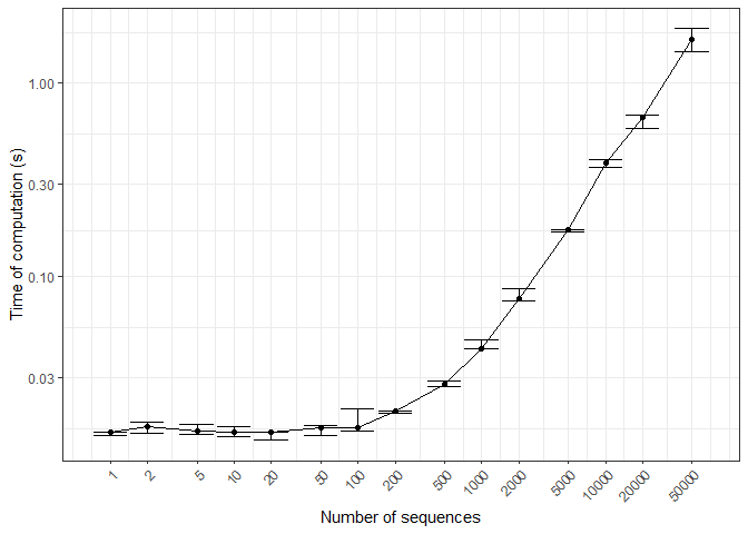
#> # ... 3 more rows in transition matrix ...The core functions of markovmix are written with
Rcpp to efficiently process sequences and probabilities.
Here, time of computation (ToC) is profiled with the number of
sequences, where dots correspond to ToC medians and error bars to ToC
quantiles.
# Define sequence lengths for ToC profiling
mk_toc_seq_len <- as.integer(outer(c(1L, 2L, 5L), 10^(seq_len(5L) - 1L)))
set.seed(4444L)
mk_toc_seq_list <- purrr::map(
  mk_toc_seq_len,
  ~ gen_seq_list(size = .x, len_range = mk_len_range, states = mk_states)
)
mk_toc_clusters <- purrr::map(
  mk_toc_seq_len,
  ~ matrix(runif(.x * mk_n_comp), nrow = .x, ncol = mk_n_comp)
)
mk_toc_exprs <- purrr::map(
  purrr::set_names(seq_along(mk_toc_seq_len), mk_toc_seq_len),
  ~ rlang::expr(fit_markov_mix(
    seq_list = mk_toc_seq_list[[!!.x]],
    order. = 2L,
    states = mk_states,
    clusters = mk_toc_clusters[[!!.x]],
    verbose = FALSE
  ))
)
# Profile time of computation
mk_toc <- bench::mark(
  exprs = mk_toc_exprs,
  min_time = Inf,
  iterations = 5L,
  filter_gc = FALSE,
  check = FALSE
)
mk_toc_plot_data <- mk_toc %>%
tibble::as_tibble() %>%
dplyr::select(expression, time) %>%
dplyr::rename(seq_len = expression, toc = time) %>%
dplyr::mutate_at("seq_len", ~ as.integer(names(.x))) %>%
dplyr::mutate_at("toc", ~ purrr::map(.x, unclass)) %>%
tidyr::unnest("toc")
ggplot2::ggplot(mk_toc_plot_data %>%
dplyr::group_by(seq_len) %>%
dplyr::summarize(toc_median = median(toc, na.rm = TRUE),
toc_min = quantile(toc, 0.25, na.rm = TRUE),
toc_max = quantile(toc, 0.75, na.rm = TRUE),
.groups = "drop"),
ggplot2::aes(x = seq_len, y = toc_median)) +
ggplot2::geom_line() +
ggplot2::geom_point() +
ggplot2::geom_errorbar(ggplot2::aes(ymin = toc_min, ymax = toc_max)) +
ggplot2::scale_x_log10(breaks = mk_toc_seq_len) +
ggplot2::scale_y_log10() +
ggplot2::theme_bw() +
ggplot2::theme(axis.text.x = ggplot2::element_text(angle = 45, hjust = 1, vjust = 1)) +
ggplot2::labs(x = "Number of sequences", y = "Time of computation (s)")