ibdsim2

Try the online app for visualising IBD distributions: ibdsim2-shiny

Introduction

The purpose of ibdsim2 is to simulate and analyse the gene flow in pedigrees. In particular, such simulations can be used to study distributions of chromosomal segments shared identical-by-descent (IBD) by pedigree members. In each meiosis, the recombination process is simulated using sex specific recombination rates in the human genome (Halldorsson et al., 2019), or with recombination maps provided by the user. Additional features include calculation of realised relatedness coefficients, distribution plots of IBD segments, and estimation of two-locus relatedness coefficients.

ibdsim2 is part of the ped suite collection of packages for pedigree analysis in R. A detailed presentation of these packages, including a separate chapter on ibdsim2, is available in the book Pedigree analysis in R (Vigeland, 2021).

Installation

To get ibdsim2, install from CRAN as follows:

install.packages("ibdsim2")

Alternatively, the latest development version can be installed from GitHub:

# install.packages("devtools") # if needed
devtools::install_github("magnusdv/ibdsim2")

Example 1: A simple simulation

The most important function in ibdsim2 is ibdsim(), which simulates the recombination process in a given pedigree. In this example we demonstrate this for in a family quartet, and show how to visualise the result.

We start by loading ibdsim2.

library(ibdsim2)

The main input to ibdsim() is a pedigree and a recombination map. In our case we use pedtools::nuclearPed() to create the pedigree, and we load chromosome 1 of the built-in map of human recombination.

# Pedigree with two siblings
x = nuclearPed(2)

# Recombination map
chr1 = loadMap("decode19", chrom = 1)

Now run the simulation! The seed argument ensures reproducibility.

sim = ibdsim(x, N = 1, map = chr1, seed = 1234, verbose = F)

The output of ibdsim() is a matrix (or a list of matrices, if N > 1). Here are the first few rows of the simulation we just made:

head(sim)
#>      chrom   startMB      endMB   startCM      endCM 1:p 1:m 2:p 2:m 3:p 3:m 4:p 4:m
#> [1,]     1  1.431813   2.933317  0.000000   1.594905   1   2   3   4   1   3   2   4
#> [2,]     1  2.933317  17.311158  1.594905  32.879029   1   2   3   4   2   3   2   4
#> [3,]     1 17.311158  20.230184 32.879029  40.490928   1   2   3   4   2   3   2   3
#> [4,]     1 20.230184  54.938719 40.490928  77.308688   1   2   3   4   2   3   2   4
#> [5,]     1 54.938719  58.982628 77.308688  83.152790   1   2   3   4   2   4   2   4
#> [6,]     1 58.982628 159.794234 83.152790 154.725693   1   2   3   4   1   4   2   4

Each row of the matrix corresponds to a segment of the genome, and describes the allelic state of the pedigree in that segment. Each individual has two columns, one with the paternal allele (marked by the suffix “:p”) and one with the maternal (suffix “:m”). The founders (the parents in our case) are assigned alleles 1, 2, 3 and 4.

The function haploDraw() interprets the founder alleles as colours and draws the resulting haplotypes onto the pedigree. See ?haploDraw for an explanation of pos and other arguments.

haploDraw(x, sim, pos = c(2, 4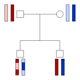, 1, 1))

Example 2: Distributions of IBD segments

In this example we will compare the distributions of counts/lengths of IBD segments between the following pairwise relationships:

• Grandparent/grandchild (GR)
• Half siblings (HS)
• Half uncle/nephew (HU)

Note that GR and HS have the same relatedness coefficients kappa = (1/2, 1/2, 0), meaning that they are genetically indistinguishable in the context of unlinked loci. In contrast, HU has kappa = (3/4, 1/4, 0).

For simplicity we create a pedigree containing all the three relationships we are interested in.

x = halfSibPed() |> addSon(5)
plot(x)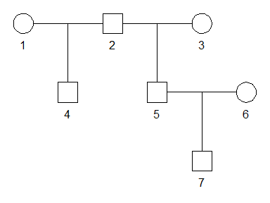

We store the ID labels of the three relationships in a list.

ids = list(GR = c(2,7), 
           HS = 4:5, 
           HU = c(4,7))

Next, we use ibdsim() to produce 500 simulations of the underlying IBD pattern in the entire pedigree.

s = ibdsim(x, N = 500, map = "decode19", seed = 1234)
#> Simulation parameters:
#> Simulations  : 500
#> Chromosomes  : 1-22
#> Genome length: 2753.93 Mb
#>                2602.29 cM (male)
#>                4180.42 cM (female)
#> Recomb model : chi
#> Target indivs: 1-7
#> Skip recomb  : -
#> Total time used: 6.27 secs

The plotSegmentDistribution() function, with the option type = "ibd1" analyses the IBD segments in each simulation, and makes a nice plot. Note that the names of the ids list are used in the legend.

plotSegmentDistribution(s, type = "ibd1", ids = ids, shape = 1:3)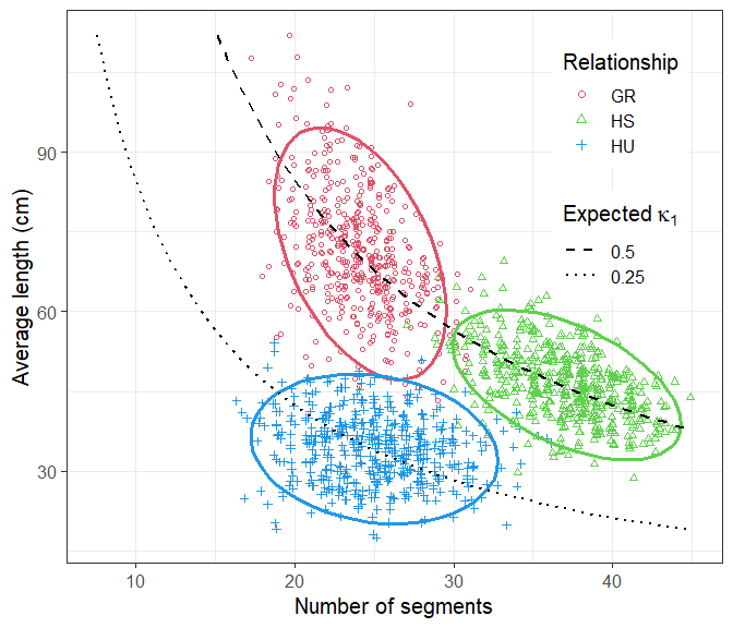

We conclude that the three distributions are almost completely disjoint. Hence the three relationships can typically be distinguished on the basis of their IBD segments, if these can be determined accurately enough.

A Shiny app for visualising IBD distributions is now available here: https://magnusdv.shinyapps.io/ibdsim2-shiny/.