![]()
![]()
The goal of the ggplate package is to enable users to create simple plots of biological culture plates as well as microplates. Both continuous and discrete values can be plotted onto the plate layout.
Currently the package supports the following plate sizes:
ggplate is implemented as an R package.
You can install the release version from CRAN using the
install.packages() function.
install.packages("ggplate")You can install the development version from GitHub using the devtools
package by copying the following commands into R:
Note: If you do not have devtools installed make sure to
do so by removing the comment sign (#).
# install.packages("devtools")
devtools::install_github("jpquast/ggplate")
In addition, you can install it via the command line through
conda since it is also implemented as a conda-forge
package.
conda install -c conda-forge r-ggplateIn order to use ggplate you have to load the package
in your R environment by simply calling the library()
function as shown bellow.
# Load ggplate package
library(ggplate)
There are multiple example datasets provided that can be used to
create plots of each plate type. You can access these datasets using the
data() function.
# Load a dataset of continuous values for a 96-well plate
data(data_continuous_96)

# Check the structure of the dataset
str(data_continuous_96)
#> Classes 'tbl_df', 'tbl' and 'data.frame':    96 obs. of  2 variables:
#>  $ Value: num  1.19 0.88 0.17 0.85 0.78 0.23 1.95 0.4 0.88 0.26 ...
#>  $ well : chr  "A1" "A2" "A3" "A4" ...
When calling the str() function you can see that the
data frame of a continuous 96-well plate dataset only contains two
columns. The Value column contains values associated with
each of the plate wells, while the well column contains the
corresponding well positions using a combination of alphabetic
row names and numeric column names.
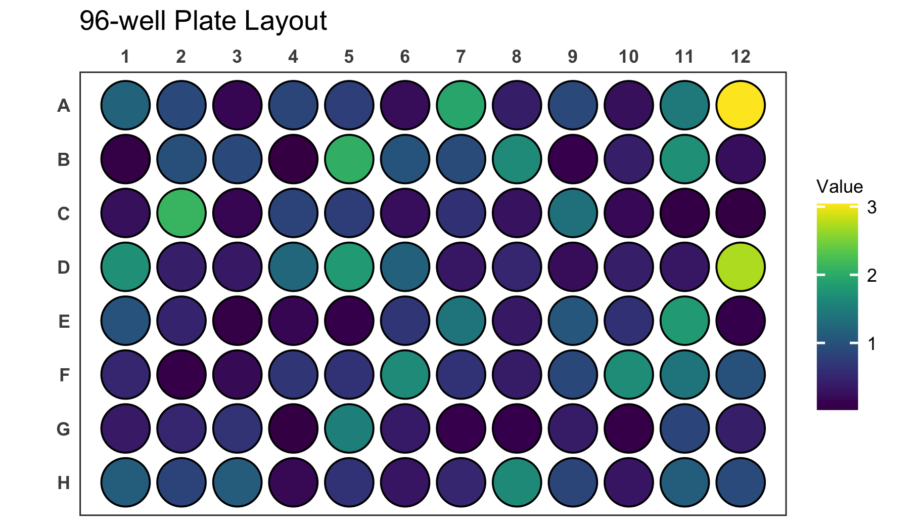
You can use this example data frame to create a 96-well plate layout
plot using the plate_plot() function and setting the
plate_size argument to 96. There are currently
two options for the plate well type. These can be either
"round" or "square". In the plot below we
specify "round", while "square" is the default
value when the plate_type argument is not provided.
The data frame is provided to the data argument and the
column name of the column containing the well positions is provided to
the position argument. The column name of the column
containing the values is provided to the value
argument.
Note: For an R markdown file set the chunk options to
dpi=300 for an optimal result.
# Create a 96-well plot with round wells
plate_plot(
  data = data_continuous_96,
  position = well,
  value = Value,
  plate_size = 96,
  plate_type = "round"
)
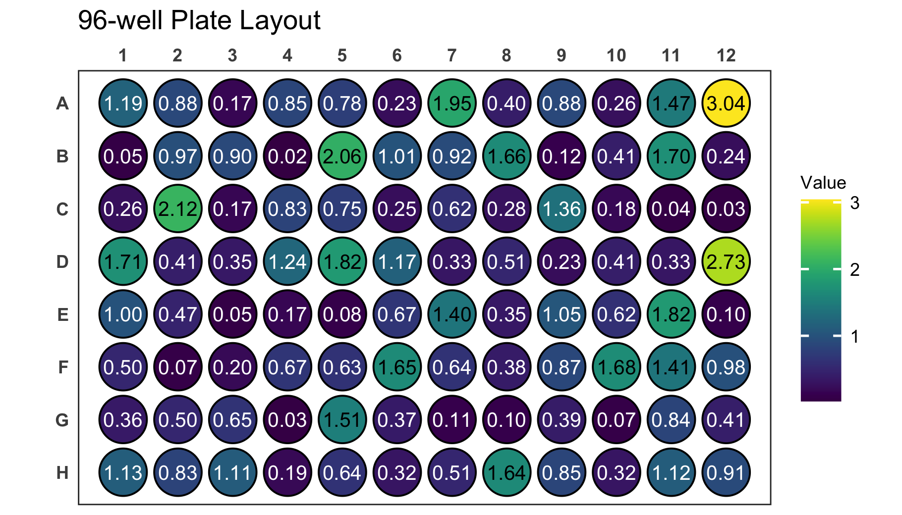
It is also possible to label each well in the plate with a
corresponding label. For the plate above it would be interesting to
display the exact value on each of the wells in addition to the
colouring. For that we use the label argument which takes
the name of the column containing the label as an input. In this example
case this column is the same that is also provided to the
value argument.
# Create a 96-well plot with labels
plate_plot(
  data = data_continuous_96,
  position = well,
  value = Value,
  label = Value,
  plate_size = 96,
  plate_type = "round"
)
Try providing the well column to the label
argument instead of the Value column. This will label each
will with its position, which might make it easier to find specific
positions.
# Create a 96-well plot with labels
plate_plot(
  data = data_continuous_96,
  position = well,
  value = Value,
  label = well,
  plate_size = 96,
  plate_type = "round"
)
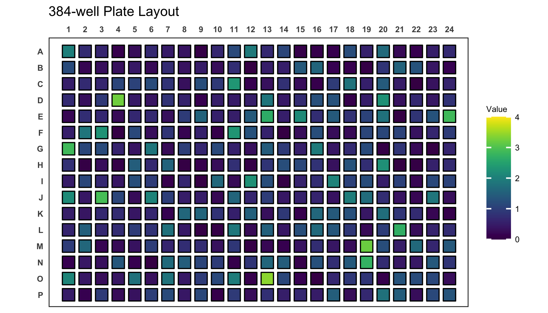
The legend for continuous values will only cover a range from the
minimal measured to the maximal measured value. If the theoretically
expected range of values is however bigger than the measured range you
can adjust the legend limits. This can be done using the
limits arguments. You provide a vector with the new minimum
and maximum to the argument. Use NA to refer to the existing minimum or
maximum if you only want to adjust one. Below we show this for an
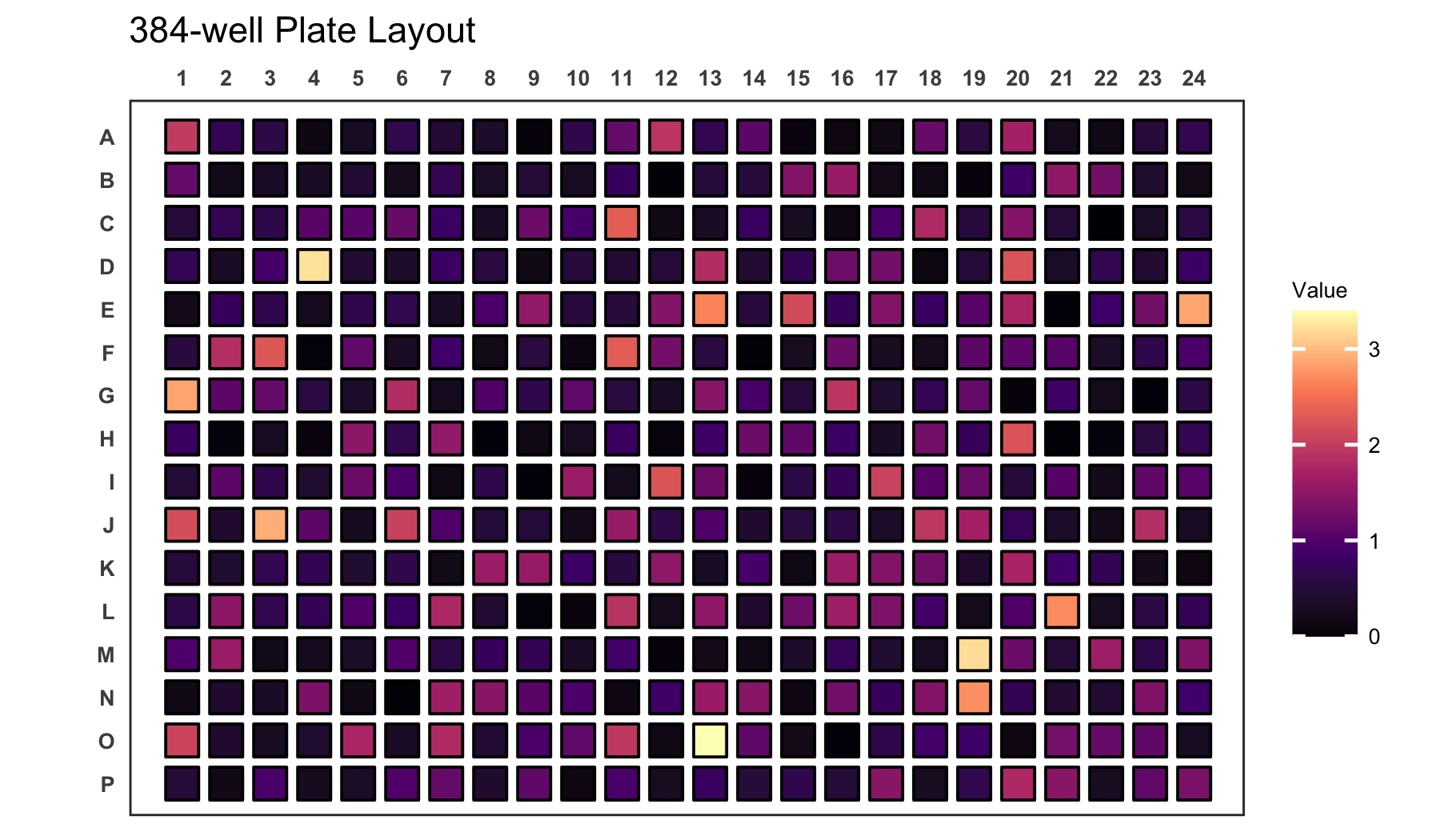
example dataset of a 384-well plate.
# Load a dataset of continuous values for a 384-well plate
data(data_continuous_384)

# Check the structure of the dataset
str(data_continuous_384)
#> tibble [384 × 2] (S3: tbl_df/tbl/data.frame)
#>  $ Value: num [1:384] 1.98 0.7 0.61 0.12 0.27 0.67 0.47 0.37 0.04 0.65 ...
#>  $ well : chr [1:384] "A1" "A2" "A3" "A4" ...

# Create a 384-well plot with adjusted legend limits
plate_plot(
  data = data_continuous_384,
  position = well,
  value = Value,
  plate_size = 384,
  limits = c(0, 4)
)
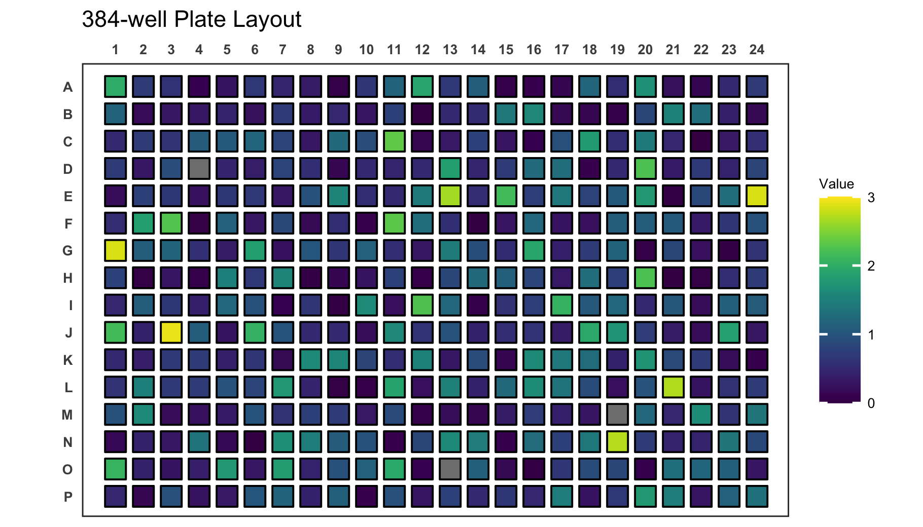
If your new range will be smaller than the measured range, values outside of the range are coloured gray.
# Create a 384-well plot with adjusted legend limits and outliers
plate_plot(
  data = data_continuous_384,
  position = well,
  value = Value,
  plate_size = 384,
  limits = c(0, 3)
)
When plotting continuous variables it is possible to to change the
gradient colours by providing new colours to the colour
argument. The colours will be used to create a new colour gradient for
the plot.
# Create a 384-well plot with a new colour gradient
plate_plot(
  data = data_continuous_384,
  position = well,
  value = Value,
  plate_size = 384,
  colour = c(
    "#000004FF",
    "#51127CFF",
    "#B63679FF",
    "#FB8861FF",
    "#FCFDBFFF"
  )
)
If you have a dataset that does not contain a value for each well,
empty wells will be uncoloured. Empty wells can either contain
NA as their value argument or they can be
completely omitted from the input data frame.
# Load a continuous of discrete values for a 48-well plate
data(data_continuous_48_incomplete)

# Check the structure of the dataset
str(data_continuous_48_incomplete)
#> tibble [48 × 2] (S3: tbl_df/tbl/data.frame)
#>  $ Value: num [1:48] 1.14 0.46 0.72 0.17 NA NA NA NA 1.37 0.37 ...
#>  $ well : chr [1:48] "A1" "A2" "A3" "A4" ...

# Create a 48-well plot with adjusted legend limits
plate_plot(
  data = data_continuous_48_incomplete,
  position = well,
  value = Value,
  plate_type = "round",
  plate_size = 48
)![]()
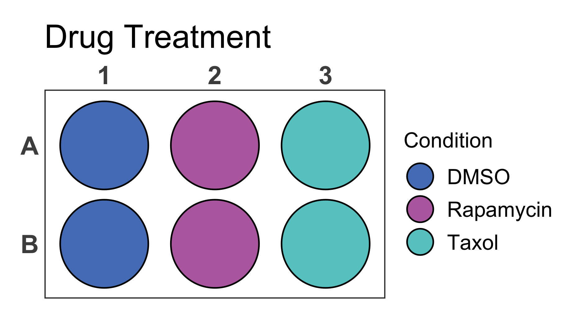
You can further customise your plot in various ways. Lets take a discrete 6-well plate dataset as an example. This dataset only contains three categories assigned to the six wells of the plate. This could be for example a pipetting scheme of an experiment.
You can change the title of the plot using the title
argument. In addition the size of the title can be adjusted using the
title_size argument.
Note: Using the R markdown chunk options out.width
and fig.align you can reduce the size of the figure in the
R markdown document and align it for example to the center.
# Load a dataset of discrete values for a 6-well plate
data(data_discrete_6)

# Check the structure of the dataset
str(data_discrete_6)
#> tibble [6 × 2] (S3: tbl_df/tbl/data.frame)
#>  $ Condition: chr [1:6] "DMSO" "Rapamycin" "Taxol" "DMSO" ...
#>  $ well     : chr [1:6] "A1" "A2" "A3" "B1" ...

# Create a 6-well plot with new title
plate_plot(
  data = data_discrete_6,
  position = well,
  value = Condition,
  plate_size = 6,
  plate_type = "round",
  title = "Drug Treatment",
  title_size = 23
)
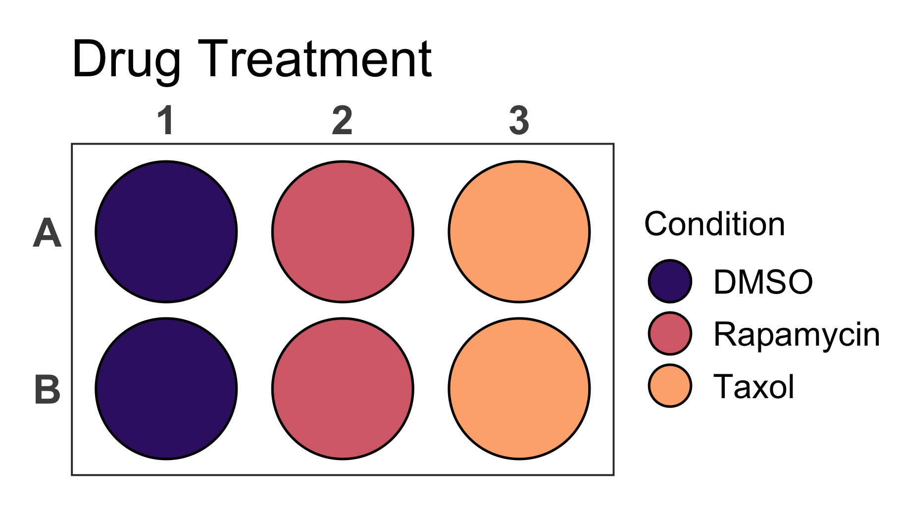
In addition it is possible to change the colours of the plot by
providing new colours to the colour argument. As mentioned
earlier this does not only work for discrete values but also for
gradients that will be created based on the provided colours.
# Create a 6-well plot
plate_plot(
  data = data_discrete_6,
  position = well,
  value = Condition,
  plate_size = 6,
  plate_type = "round",
  title = "Drug Treatment",
  title_size = 23,
  colour = c("#3a1c71", "#d76d77", "#ffaf7b")
)
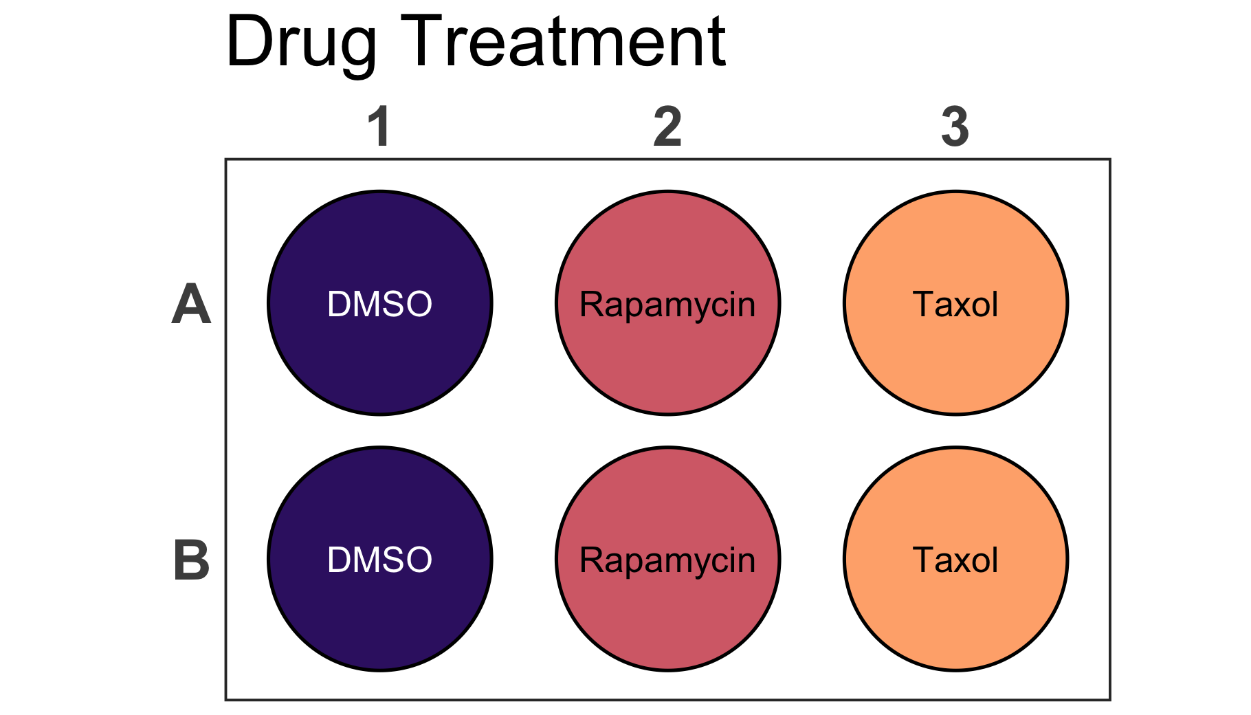
Also for this plot we can provide a column name to the
label argument to directly label the wells in the plot. At
the same time we can disable the legend setting the
show_legend argument to FALSE. In this case
the labels for each well are too large and we should also resize the
label so that it fits perfectly into each well using the
label_size argument.
# Create a 6-well plot
plate_plot(
  data = data_discrete_6,
  position = well,
  value = Condition,
  label = Condition,
  plate_size = 6,
  plate_type = "round",
  title = "Drug Treatment",
  title_size = 23,
  colour = c("#3a1c71", "#d76d77", "#ffaf7b"),
  show_legend = FALSE,
  label_size = 4
)
In order to have the same proportions independent on the output
screen and size, each plate plot is scaled according to the specific
graphics device size. In order to see the currently used graphics device
size and scaling factor the silent argument of the function
can be set to FALSE.
As you can see for the bellow example the graphics device size is
width: 7 height: 4 and the scaling factor is
1.256.
# Load a dataset of discrete values for a 24-well plate
data(data_discrete_24)

# Check the structure of the dataset
str(data_discrete_24)
#> tibble [24 × 2] (S3: tbl_df/tbl/data.frame)
#>  $ Condition: chr [1:24] "siControl" "siRaptor" "siRagB" "siRagD" ...
#>  $ well     : chr [1:24] "A1" "A2" "A3" "A4" ...

# Create a 24-well plot
plate_plot(
  data = data_discrete_24,
  position = well,
  value = Condition,
  plate_size = 24,
  plate_type = "round",
  silent = FALSE
)
#> width: 7 height: 4
#> scaling factor: 1.256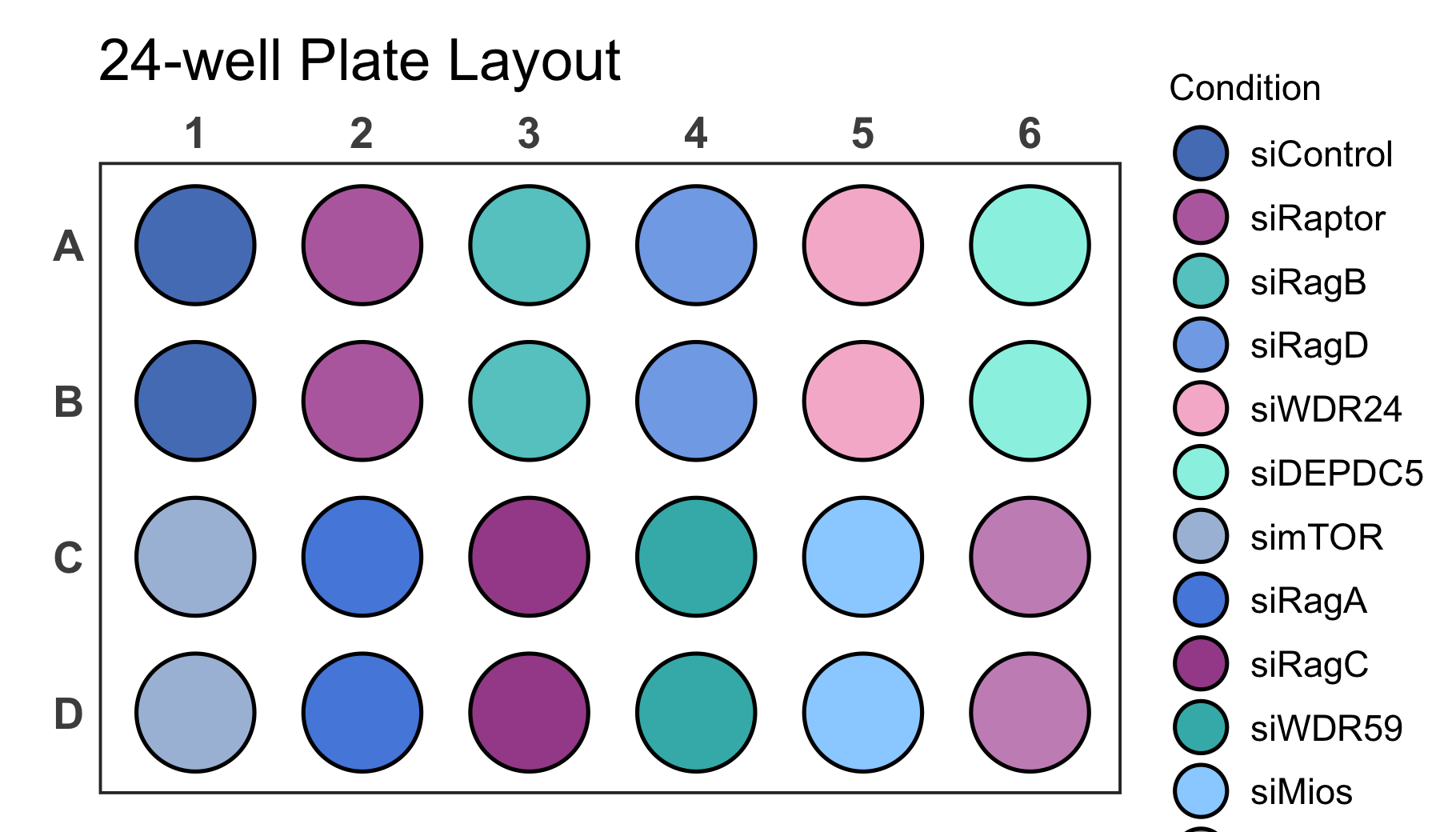
It is possible that the generated plot has overlapping or too spaced
out wells. This can be corrected by resizing the output graphics device
size until the plot has the desired proportions. If a specific output
size is required and the plot does not have the desired proportions you
can use the scale argument to adjust it as shown below.
Note: If you run the package directly in the command line, the
function opens a new graphics device since it is not already opened like
it would be the case in RStudio. If this is not desired you can avoid
this by setting the scale argument.
# Create a 24-well plot
plate_plot(
  data = data_discrete_24,
  position = well,
  value = Condition,
  plate_size = 24,
  plate_type = "round",
  silent = FALSE,
  scale = 1.45
)
#> width: 7 height: 4
#> scaling factor: 1.45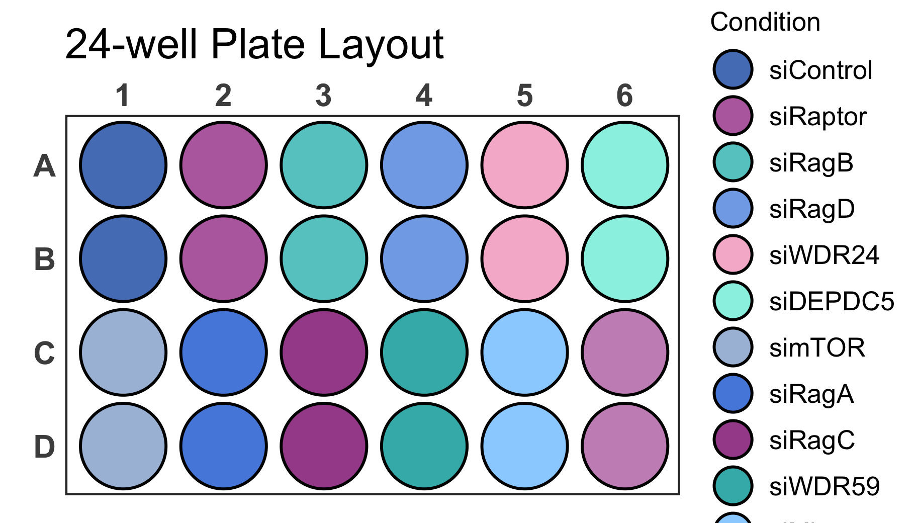
As you can see, however, now we are running into the problem that the
legend is larger than the screen size. With the
legend_n_row argument you can manually determine the number
of rows that should be used for the legend. In this case it is ideal to
split the legend into 2 columns by setting legend_n_row to
6 rows. In addition we should adjust the scale parameter to
1.2 in order to space out wells properly.
# Create a 24-well plot with 2 row legend
plate_plot(
  data = data_discrete_24,
  position = well,
  value = Condition,
  plate_size = 24,
  plate_type = "round",
  silent = FALSE,
  scale = 1.2,
  legend_n_row = 6
)
#> width: 7 height: 4
#> scaling factor: 1.2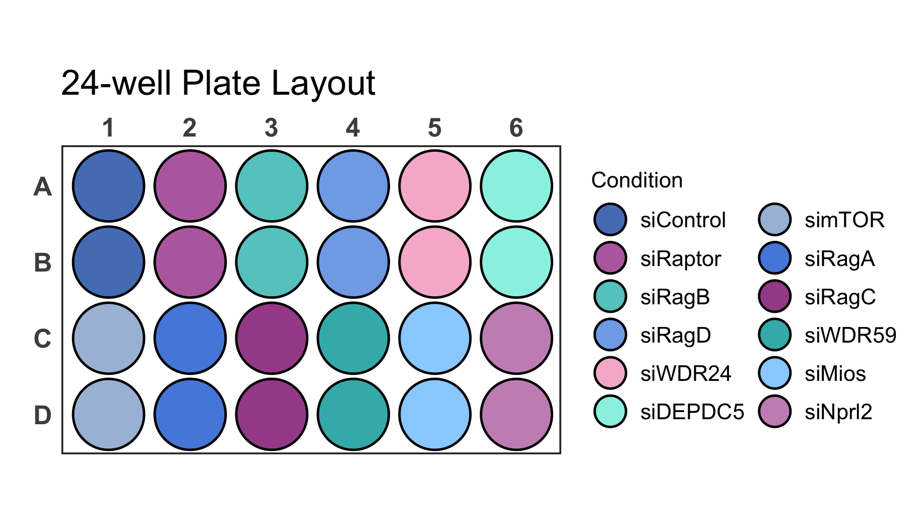
If your dataset has a lot of labels it can become difficult to impossible to distinguish them just by colour as you can see for the dataset below.
# Load a dataset of discrete values for a 96-well plate
data(data_discrete_96)

# Check the structure of the dataset
str(data_discrete_96)
#> tibble [96 × 3] (S3: tbl_df/tbl/data.frame)
#>  $ Compound          : chr [1:96] "Positive Control" "Axitinib" "Gefitinib (ZD1839)" "Rapamycin (Sirolimus)" ...
#>  $ well              : chr [1:96] "A1" "A2" "A3" "A4" ...
#>  $ Compound_multiline: chr [1:96] "Positive\nControl" "Axitinib" "Gefitinib\n(ZD1839)" "Rapamycin\n(Sirolimus)" ...

# Create a 96-well plot
plate_plot(
  data = data_discrete_96,
  position = well,
  value = Compound,
  plate_size = 96,
  scale = 0.95,
  plate_type = "round"
)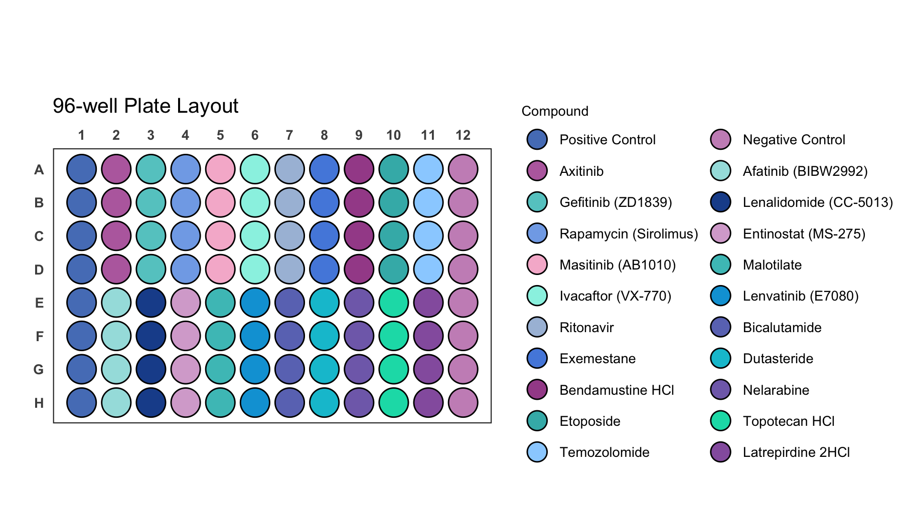
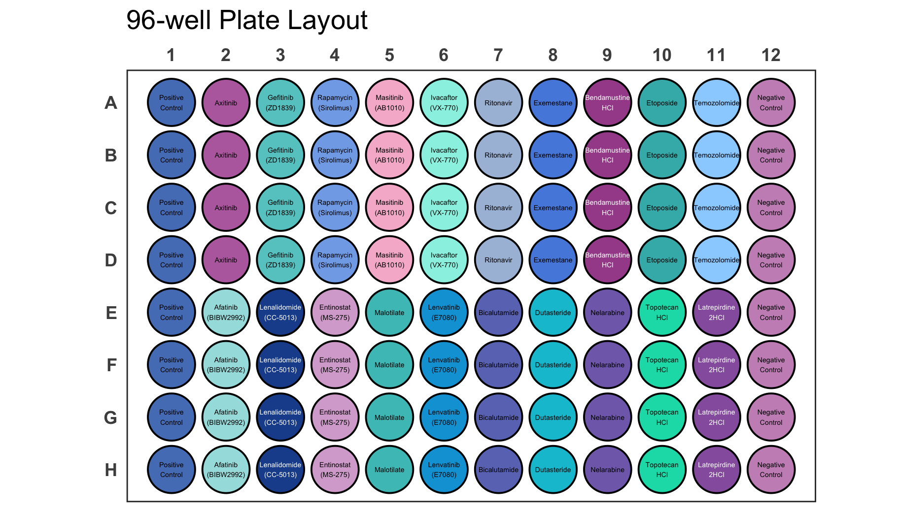
This is an example where it is likely better to directly label wells instead of displaying a legend.
# Create a 96-well plot with labels
plate_plot(
  data = data_discrete_96,
  position = well,
  value = Compound,
  label = Compound_multiline, # using a column that contains line brakes for labeling
  plate_size = 96,
  show_legend = FALSE, # hiding legend
  label_size = 1.1, # setting label size
  plate_type = "round"
)
Since the plot function checks the size of the graphics device in
order to apply the appropriate scaling to the plot, it is important to
first generate an output graphics device with the correct size. There
are several functions that can accomplish this. These include
e.g. png(), pdf(), svg() and many
more.
# Generate a new graphics device with a defined size
png("plate_plot_384_well_plate.png", width = 10, height = 6, unit = "in", res = 300)

# Create a plot
plate_plot(
  data = data_continuous_384,
  position = well,
  value = Value,
  label = Value,
  plate_size = 384,
  colour = c(
    "#000004FF",
    "#51127CFF",
    "#B63679FF",
    "#FB8861FF",
    "#FCFDBFFF"
  )
)

# Close graphics device
dev.off()