
![]()
The gdm package provides functions to fit, plot,
summarize, and apply Generalized Dissimilarity Models.
The gdm package is available on CRAN, development versions are available on GitHub.
install.packages("gdm")if (!require("devtools")) {
install.packages("devtools")
}
devtools::install_github("fitzLab-AL/gdm")Fitzpatrick MC, Mokany K, Manion G, Nieto-Lugilde D, Ferrier S. (2024) gdm: Generalized Dissimilarity Modeling. R package version 1.6.
The gdm package has been updated to leverage the terra
package as its raster processing engine, leading to faster raster file
processing. Preferably, inputs should be provided as
SpatRaster objects, or any convertible object to
terra, such as raster
package objects or stars
objects.
With the transition to terra, the gdm
package is now capable of efficiently handling very large raster files,
thanks to the underlying terra functionalities. Memory
management is handled automatically by terra, but in the
event of encountering out-of-memory errors, you can utilize
terra::terraOptions(steps = ...) to increase the number of
processing steps for large files.
GDM has been used in many published studies. In addition to working through the examples here and those throughout the package documentation, we recommend reading these publications for background information:
Ferrier S, Manion G, Elith J, Richardson, K (2007) Using generalized dissimilarity modelling to analyse and predict patterns of beta diversity in regional biodiversity assessment. Diversity & Distributions 13: 252-264.https://doi.org/10.1111/j.1472-4642.2007.00341.x
Mokany K, Ware C, Woolley, SNC, Ferrier S, Fitzpatrick MC (2022) A working guide to harnessing generalized dissimilarity modelling for biodiversity analysis and conservation assessment. Global Ecology and Biogeography, 31, 802– 821. https://doi.org/10.1111/geb.13459
The R package gdm implements Generalized Dissimilarity Modeling Ferrier et al. 2007 to analyze and map spatial patterns of biodiversity. GDM models biological variation as a function of environment and geography using distance matrices – specifically by relating biological dissimilarity between sites to how much sites differ in their environmental conditions (environmental distance) and how isolated they are from one another (geographical distance). Here we demonstrate how to fit, apply, and interpret GDM in the context of analyzing and mapping species-level patterns. GDM also can be used to model other biological levels of organization, notably genetic Fitzpatrick & Keller 2015, phylogenetic Rosauer et al. 2014, or function/traits Thomassen et al. 2010, and the approaches for doing so are largely identical to the species-level case with the exception of using a different biological dissimilarity metric depending on the type of response variable.
The initial step in fitting a generalized dissimilarity model is to
combine the biological and environmental data into “site-pair” table
format using the formatsitepair function.
GDM can use several data formats as input. Most common are site-by-species tables (sites in rows, species across columns) for the response and site-by-environment tables (sites in rows, predictors across columns) as the predictors, though distance matrices and rasters also are accommodated as demonstrated below.
The gdm package comes with two example biological
data sets and two example environmental data sets in a number of
formats. Example data include: - southwest: A data frame
that contains x-y coordinates, 10 columns of predictors (five soil and
five bioclimatic variables), and occurrence data for 900+ species of
plants from southwest Australia (representing a subset of the data used
in [@fitzpatrick_2013]). Note that the
format of the southwest table is an x-y species list (i.e.,
bioFormat = 2, see below) where there is one row per
species record rather than per site. These biological data are
similar to what would be obtained from online databases such as GBIF. - gdmDissim: A
pairwise biological dissimilarity matrix derived from the species data
provided in southwest. gdmDissim is provided
to demonstrate how to proceed when you when you want to fit GDM using an
existing biological distance matrix (e.g., pairwise Fst) as the response
variable (i.e., bioFormat = 3, see below). Note however
that distance matrices can also be used as predictors (e.g., to model
compositional variation in one group as a function of compositional
variation in another group Jones et al 2013. -
swBioclims: a raster stack of the five bioclimatic
predictors provided in the southwest data.
Note that for all input data the rows and their order must match in the biological and environmental data frames and must not include NAs. This is best accomplished by making sure your tables have a column with a unique identifier for each site and that the order of these IDs are the same across all tables.
To build a site-pair table, we need individual tables for the
biological and environmental data, so we first index the
southwest table to create a table for the species data and
a second for the environmental data:
library(gdm)
# have a look at the southwest data set
str(southwest)
#> 'data.frame':    29364 obs. of  14 variables:
#>  $ species   : Factor w/ 974 levels "spp1","spp10",..: 1 1 1 1 1 1 1 1 1 1 ...
#>  $ site      : int  1066 1026 1025 1026 1027 1047 1048 1066 1066 1067 ...
#>  $ awcA      : num  14.5 16.3 23.1 16.3 17 ...
#>  $ phTotal   : num  546 471 460 471 489 ...
#>  $ sandA     : num  71.3 68.9 71.5 68.9 74.7 ...
#>  $ shcA      : num  178.9 105.8 88.4 105.8 147.2 ...
#>  $ solumDepth: num  875 928 892 928 952 ...
#>  $ bio5      : num  31.4 33.1 32.8 33.1 33.2 ...
#>  $ bio6      : num  5.06 4.85 4.82 4.85 4.59 ...
#>  $ bio15     : num  40.4 48.2 53.9 48.2 44 ...
#>  $ bio18     : int  0 0 43 0 0 0 0 0 0 0 ...
#>  $ bio19     : num  133 140 145 140 136 ...
#>  $ Lat       : num  -33 -32 -32 -32 -32.1 ...
#>  $ Long      : num  119 118 118 118 119 ...

# biological data
# get columns with xy, site ID, and species data
sppTab <- southwest[, c("species", "site", "Long", "Lat")]

# # columns 3-7 are soils variables, remainder are climate
# get columns with site ID, env. data, and xy-coordinates
envTab <- southwest[, c(2:ncol(southwest))]
Because the southwest data is x-y species list format,
we use bioFormat=2. Otherwise, we just need to provide the
required column names to create the site-pair table:
# x-y species list example
gdmTab <- formatsitepair(bioData=sppTab,
                         bioFormat=2, #x-y spp list
                         XColumn="Long",
                         YColumn="Lat",
                         sppColumn="species",
                         siteColumn="site",
                         predData=envTab)
#> distance weights s1.xCoord s1.yCoord s2.xCoord s2.yCoord s1.awcA
#> 132 0.4485981 1 115.057 -29.40472 115.5677 -29.46599 23.0101
#> 132.1 0.7575758 1 115.057 -29.40472 116.0789 -29.52556 23.0101
#> 132.2 0.8939394 1 115.057 -29.40472 116.5907 -29.58342 23.0101
#> s1.phTotal s1.sandA s1.shcA s1.solumDepth s1.bio5 s1.bio6 s1.bio15
#> 132 480.3266 83.99326 477.5656 1129.933 34.668 8.908 86.64
#> 132.1 480.3266 83.99326 477.5656 1129.933 34.668 8.908 86.64
#> 132.2 480.3266 83.99326 477.5656 1129.933 34.668 8.908 86.64
#> s1.bio18 s1.bio19 s2.awcA s2.phTotal s2.sandA s2.shcA s2.solumDepth
#> 132 0 267.44 22.3925 494.1225 76.6900 357.7225 1183.9025
#> 132.1 0 267.44 17.0975 415.1275 70.0175 112.4800 985.5300
#> 132.2 0 267.44 17.0300 333.4400 71.5950 165.7250 956.5425
#> s2.bio5 s2.bio6 s2.bio15 s2.bio18 s2.bio19
#> 132 35.50571 7.448572 75.37143 0 228.6572
#> 132.1 36.05000 6.605882 64.52941 0 168.8824
#> 132.2 36.18750 6.131250 58.75000 0 141.1250The first column of a site-pair table contains a biological distance measure (the default is Bray-Curtis distance though any measure scaled between 0-1 is acceptable). The second column contains the weight to be assigned to each data point in model fitting (defaults to 1 if equal weighting is used, but can be customized by the user or can be scaled to site richness, see below). The remaining columns are the coordinates and environmental values at a site (s1) and those at a second site (s2) making up a site pair. Rows represent individual site-pairs. While the site-pair table format can produce extremely large data frames and contain numerous repeat values (because each site appears in numerous site-pairs), it also allows great flexibility. Most notably, individual site pairs easily can be excluded from model fitting.
A properly formatted site-pair table will have at least six columns
(distance, weights, s1.xCoord, s1.yCoord, s2.xCoord, s2.yCoord) and some
number more depending on how many predictors are included. See
?formatsitepair and ?gdm for more details.
What if you already have a biological distance matrix because you are
working with, say, genetic data? In that case, it is simple as changing
the bioFormat argument and providing that matrix as the
bioData object to the sitepairformat function.
However, in addition to the pairwise dissimilarity values, the object
must include a column containing the site IDs. Let’s have a quick look
at gdmDissim, a pairwise biological distance matrix
provided with the package (note that the first column contains site
IDs):
# Biological distance matrix example
dim(gdmDissim)
#> [1] 94 95
gdmDissim[1:5, 1:5]
#>    site         1         2         3         4
#> V1  881 0.0000000 0.4485981 0.7575758 0.8939394
#> V2  882 0.4485981 0.0000000 0.5837563 0.8170732
#> V3  883 0.7575758 0.5837563 0.0000000 0.4782609
#> V4  884 0.8939394 0.8170732 0.4782609 0.0000000
#> V5  885 0.9178082 0.8202247 0.5813953 0.4375000
We can provide the gdmDissim object to
formatsitepair as follows:
gdmTab.dis <- formatsitepair(bioData=gdmDissim,
                             bioFormat=3, #diss matrix
                             XColumn="Long",
                             YColumn="Lat",
                             predData=envTab,
                             siteColumn="site")
#> distance weights s1.xCoord s1.yCoord s2.xCoord s2.yCoord s1.awcA
#> 132 0.4485981 1 115.057 -29.40472 115.5677 -29.46599 23.0101
#> 132.1 0.7575758 1 115.057 -29.40472 116.0789 -29.52556 23.0101
#> 132.2 0.8939394 1 115.057 -29.40472 116.5907 -29.58342 23.0101
#> s1.phTotal s1.sandA s1.shcA s1.solumDepth s1.bio5 s1.bio6 s1.bio15
#> 132 480.3266 83.99326 477.5656 1129.933 34.668 8.908 86.64
#> 132.1 480.3266 83.99326 477.5656 1129.933 34.668 8.908 86.64
#> 132.2 480.3266 83.99326 477.5656 1129.933 34.668 8.908 86.64
#> s1.bio18 s1.bio19 s2.awcA s2.phTotal s2.sandA s2.shcA s2.solumDepth
#> 132 0 267.44 22.3925 494.1225 76.6900 357.7225 1183.9025
#> 132.1 0 267.44 17.0975 415.1275 70.0175 112.4800 985.5300
#> 132.2 0 267.44 17.0300 333.4400 71.5950 165.7250 956.5425
#> s2.bio5 s2.bio6 s2.bio15 s2.bio18 s2.bio19
#> 132 35.50571 7.448572 75.37143 0 228.6572
#> 132.1 36.05000 6.605882 64.52941 0 168.8824
#> 132.2 36.18750 6.131250 58.75000 0 141.1250In addition to starting with tablular data, environmental data can be
extracted directly from rasters, assuming the x-y coordinates of sites
are provided in either a site-species table (bioFormat=1)
or as a x-y species list (bioFormat=2).
# environmental raster data for sw oz
swBioclims <- terra::rast(system.file("./extdata/swBioclims.grd", package="gdm"))

gdmTab.rast <- formatsitepair(bioData=sppTab,
                              bioFormat=2, # x-y spp list
                              XColumn="Long",
                              YColumn="Lat",
                              sppColumn="species",
                              siteColumn="site",
                              predData=swBioclims) #raster stack
Because some sites might not overlap with the rasters, we should check for and remove NA values from the site-pair table:
sum(is.na(gdmTab.rast))
#> [1] 465
gdmTab.rast <- na.omit(gdmTab.rast)
Note that the formatsitepair function assumes that the
coordinates of the sites are in the same coordinate system as the
rasters. At present, no checking is performed to ensure this is the
case. Note also that if your site coordinates are longitude-latitude
that the calculation of geographic distances between sites will have
errors, the size of which will depend on the geographic extent and
location of your study region. We hope to deal with this in a later
release, but for now you can avoid these problems by using a projected
coordinate system (e.g., equidistant).
The ideal biological data for fitting a GDM are occurrence records (presence-absence or abundance) from a network of sites where all species (from one or more taxonomic groups) have been intensively sampled such that compositional dissimilarity can be reliably estimated between sites. However most species data are collected as part of ad hoc surveys and are presence-only. Under these circumstances, there is no systematic surveying and no sites per se, but rather grid cells with some number of occurrence records depending on the number of species observed, with many grid cells having none, a few, or even a single species record. When these data are used to calculate compositional dissimilarity, erroneously high values will result, which will bias the model.
The formatsitepair function provides a few options for
dealing with this potential bias, including (i) weighting sites relative
to the number of species observed (weightType="richness"),
(ii) removing sites with few species (e.g.,
speciesFilter=10) or (iii) both. Decisions regarding which
approach to use will depend on the nature of the data and study system.
See Ferrier et al. (2007) for further discussion.
# weight by site richness using weightType="richness"
gdmTab.rw <- formatsitepair(bioData=sppTab,
                            bioFormat=2,
                            XColumn="Long",
                            YColumn="Lat",
                            sppColumn="species",
                            siteColumn="site",
                            predData=envTab,
                            weightType="richness")

# weights based on richness (number of species records)
gdmTab.rw[1:5, 1:5]
#>        distance   weights s1.xCoord s1.yCoord s2.xCoord
#> 132   0.4485981 0.2449866   115.057 -29.40472  115.5677
#> 132.1 0.7575758 0.1916207   115.057 -29.40472  116.0789
#> 132.2 0.8939394 0.1635852   115.057 -29.40472  116.5907
#> 132.3 0.9178082 0.1858930   115.057 -29.40472  117.1029
#> 132.4 0.9787234 0.1337957   115.057 -29.40472  117.6156
# remove sites with < 10 species records using
# sppFilter = 10
gdmTab.sf <- formatsitepair(bioData=sppTab,
bioFormat=2,
XColumn="Long",
YColumn="Lat",
sppColumn="species",
siteColumn="site",
predData=envTab,
sppFilter=10)GDM is a nonlinear extension of permutational matrix regression that uses flexible splines and generalized linear modeling (GLM) to accommodate two types of nonlinearity common in ecological datasets: (1) variation in the rate of compositional turnover (non-stationarity) along environmental gradients, and (2) the curvilinear relationship between biological distance and environmental and geographical distance.
The function gdm fits generalized dissimilarity models
and is simple to use once the biological and predictor data have been
formatted to a site-pair table. In addition to specifying whether or not
the model should be fit with geographical distance as a predictor
variable, the user has the option to specify (i) the number of I-spline
basis functions (the default is three, with larger values producing more
complex splines) and (ii) the locations of “knots” along the splines
(defaults to 0 (minimum), 50 (median), and 100 (maximum) quantiles when
three I-spline basis functions are used). Even though these option are
available, using the default values for these parameters will work fine
for most applications. In other words, unless you have a good reason,
you should probably use the default settings for splines and knots. The
effects (and significance) of altering the number of splines and knot
locations has not been systematically explored.
Here we fit GDM with geo=T and default settings for all other parameters.
gdm.1 <- gdm(data=gdmTab, geo=TRUE)The summary function provides an overview of the model,
the most important items to note are:
summary(gdm.1)
#> [1]
#> [1]
#> [1] GDM Modelling Summary
#> [1] Creation Date:  Sun Sep  8 23:57:50 2024
#> [1]
#> [1] Name:  gdm.1
#> [1]
#> [1] Data:  gdmTab
#> [1]
#> [1] Samples:  4371
#> [1]
#> [1] Geographical distance used in model fitting?  TRUE
#> [1]
#> [1] NULL Deviance:  651.914
#> [1] GDM Deviance:  129.025
#> [1] Percent Deviance Explained:  80.208
#> [1]
#> [1] Intercept:  0.277
#> [1]
#> [1] PREDICTOR ORDER BY SUM OF I-SPLINE COEFFICIENTS:
#> [1]
#> [1] Predictor 1: bio19
#> [1] Splines: 3
#> [1] Min Knot: 114.394
#> [1] 50% Knot: 172.416
#> [1] Max Knot: 554.771
#> [1] Coefficient[1]: 0.941
#> [1] Coefficient[2]: 0.868
#> [1] Coefficient[3]: 0
#> [1] Sum of coefficients for bio19: 1.809
#> [1]
#> [1] Predictor 2: phTotal
#> [1] Splines: 3
#> [1] Min Knot: 277.978
#> [1] 50% Knot: 584.609
#> [1] Max Knot: 1860.37
#> [1] Coefficient[1]: 1.127
#> [1] Coefficient[2]: 0.23
#> [1] Coefficient[3]: 0
#> [1] Sum of coefficients for phTotal: 1.357
#> [1]
#> [1] Predictor 3: bio5
#> [1] Splines: 3
#> [1] Min Knot: 25.571
#> [1] 50% Knot: 32.16
#> [1] Max Knot: 36.188
#> [1] Coefficient[1]: 0.127
#> [1] Coefficient[2]: 0.453
#> [1] Coefficient[3]: 0.114
#> [1] Sum of coefficients for bio5: 0.694
#> [1]
#> [1] Predictor 4: solumDepth
#> [1] Splines: 3
#> [1] Min Knot: 705.02
#> [1] 50% Knot: 1017.628
#> [1] Max Knot: 1247.705
#> [1] Coefficient[1]: 0.682
#> [1] Coefficient[2]: 0
#> [1] Coefficient[3]: 0
#> [1] Sum of coefficients for solumDepth: 0.682
#> [1]
#> [1] Predictor 5: awcA
#> [1] Splines: 3
#> [1] Min Knot: 12.975
#> [1] 50% Knot: 22.186
#> [1] Max Knot: 50.7
#> [1] Coefficient[1]: 0
#> [1] Coefficient[2]: 0
#> [1] Coefficient[3]: 0.523
#> [1] Sum of coefficients for awcA: 0.523
#> [1]
#> [1] Predictor 6: Geographic
#> [1] Splines: 3
#> [1] Min Knot: 0.452
#> [1] 50% Knot: 2.46
#> [1] Max Knot: 6.532
#> [1] Coefficient[1]: 0.014
#> [1] Coefficient[2]: 0.372
#> [1] Coefficient[3]: 0
#> [1] Sum of coefficients for Geographic: 0.386
#> [1]
#> [1] Predictor 7: sandA
#> [1] Splines: 3
#> [1] Min Knot: 56.697
#> [1] 50% Knot: 72.951
#> [1] Max Knot: 83.993
#> [1] Coefficient[1]: 0.092
#> [1] Coefficient[2]: 0
#> [1] Coefficient[3]: 0.139
#> [1] Sum of coefficients for sandA: 0.231
#> [1]
#> [1] Predictor 8: shcA
#> [1] Splines: 3
#> [1] Min Knot: 78.762
#> [1] 50% Knot: 179.351
#> [1] Max Knot: 521.985
#> [1] Coefficient[1]: 0
#> [1] Coefficient[2]: 0.156
#> [1] Coefficient[3]: 0
#> [1] Sum of coefficients for shcA: 0.156
#> [1]
#> [1] Predictor 9: bio6
#> [1] Splines: 3
#> [1] Min Knot: 4.373
#> [1] 50% Knot: 5.509
#> [1] Max Knot: 9.224
#> [1] Coefficient[1]: 0.121
#> [1] Coefficient[2]: 0
#> [1] Coefficient[3]: 0
#> [1] Sum of coefficients for bio6: 0.121
#> [1]
#> [1] Predictor 10: bio15
#> [1] Splines: 3
#> [1] Min Knot: 29.167
#> [1] 50% Knot: 55.008
#> [1] Max Knot: 87.143
#> [1] Coefficient[1]: 0.027
#> [1] Coefficient[2]: 0
#> [1] Coefficient[3]: 0
#> [1] Sum of coefficients for bio15: 0.027
#> [1]
#> [1] Predictor 11: bio18
#> [1] Splines: 3
#> [1] Min Knot: 0
#> [1] 50% Knot: 0
#> [1] Max Knot: 52
#> [1] Coefficient[1]: 0
#> [1] Coefficient[2]: 0
#> [1] Coefficient[3]: 0
#> [1] Sum of coefficients for bio18: 0The fitted splines represent one of the most informative components
of a fitted GDM and so plotting and scrutinizing the splines is a major
part of interpreting GDM and the analyzed biological patterns. The
fitted model and I-splines can be viewed using the plot
function, which produces a multi-panel plot that includes two model
summary plots showing (i) the fitted relationship between predicted
ecological distance and observed compositional dissimilarity and (ii)
predicted versus observed biological distance, followed by a series of
panels showing each I-spline with at least one non-zero coefficient
(plotted in order by sum of the I-spline coefficients). Note that in the
example bio18 is not plotted because all three coefficients equaled zero
and so had no relationship with the response.
The maximum height of each spline indicates the magnitude of total biological change along that gradient and thereby corresponds to the relative importance of that predictor in contributing to biological turnover while holding all other variables constant (i.e., is a partial ecological distance). The spline’s shape indicates how the rate of biological change varies with position along that gradient. Thus, the splines provide insight into the total magnitude of biological change as a function of each gradient and where along each gradient those changes are most pronounced. In this example, compositional turnover is greatest along gradients of bio19 (winter precipitation) and phTotal (soil phosphorus) and most rapid near the low ends of these gradients.
length(gdm.1$predictors) # get ideal of number of panels
#> [1] 11
plot(gdm.1, plot.layout=c(4,3))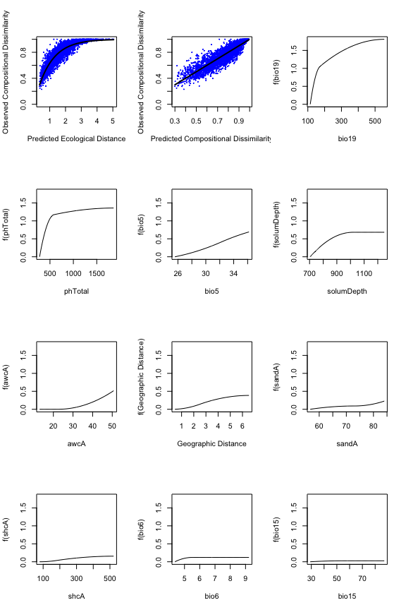
The fitted model (first two panels) and I-splines (remaining panels).
To allow easy customization of I-spline plots, the
isplineExtract function will extract the plotted values for
each I-spline.
gdm.1.splineDat <- isplineExtract(gdm.1)
str(gdm.1.splineDat)
#> List of 2
#>  $ x: num [1:200, 1:11] 0.452 0.483 0.513 0.544 0.574 ...
#>   ..- attr(*, "dimnames")=List of 2
#>   .. ..$ : NULL
#>   .. ..$ : chr [1:11] "Geographic" "awcA" "phTotal" "sandA" ...
#>  $ y: num [1:200, 1:11] 0 0.00045 0.00095 0.0015 0.0021 ...
#>   ..- attr(*, "dimnames")=List of 2
#>   .. ..$ : NULL
#>   .. ..$ : chr [1:11] "Geographic" "awcA" "phTotal" "sandA" ...
plot(gdm.1.splineDat$x[,"bio19"],
     gdm.1.splineDat$y[,"bio19"],
     lwd=3,
     type="l",
     xlab="Winter precipitation (mm)",
     ylab="Partial ecological distance")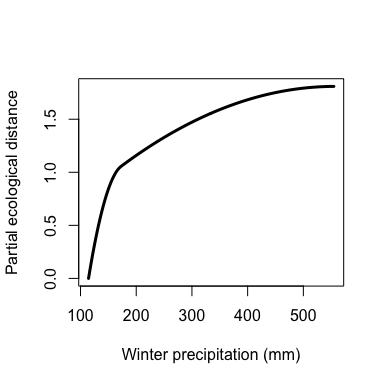
Custom I-spline plot for geographic distance.
The I-splines provide an indication of how species composition (or
any other fitted biological response variable) changes along each
environmental gradient. Beyond these insights, a fitted model also can
be used to (i) predict biological dissimilarity between site pairs in
space or between times using the predict function and (ii)
transform the predictor variables from their arbitrary environmental
scales to a common biological importance scale using the
gdm.transform function.
The following examples show predictions between site pairs in space and locations through time, and transformation of both tabular and raster data. For the raster example, the transformed layers are used to map spatial patterns of biodiversity.
The predict function requires a site-pair table in the
same format as that used to fit the model. For demonstration purposes,
we use the same table as that was used to fit the model, though
predictions to new sites (or times) can be made as well assuming the
same set of environmental/spatial predictors are available at those
locations (or times).
gdm.1.pred <- predict(object=gdm.1, data=gdmTab)

head(gdm.1.pred)
#> [1] 0.4720423 0.7133571 0.8710175 0.8534788 0.9777208 0.3996694

plot(gdmTab$distance,
     gdm.1.pred,
     xlab="Observed dissimilarity",
     ylab="Predicted dissimilarity",
     xlim=c(0,1),
     ylim=c(0,1),
     pch=20,
     col=rgb(0,0,1,0.5))
lines(c(-1,2), c(-1,2))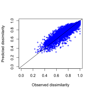
Predicted vs. observed compositional dissimilarity.
The predict function can be used to make predictions
through time, for example, under climate change scenarios to estimate
the magnitude of expected change in biological composition in response
to environmental change [@fitzpatrick_2011]. In this case,
rasters must be provided for two time periods of interest.
First we fit a new model using only the climate variables and then create some fake future climate rasters to use as example data.
# fit a new gdm using a table with climate data only (to match rasters)
gdm.rast <- gdm(gdmTab.rast, geo=TRUE)

# make some fake climate change data
futRasts <- swBioclims
##reduce winter precipitation by 25% & increase temps
futRasts[[3]] <- futRasts[[3]]*0.75
futRasts[[4]] <- futRasts[[4]]+2
futRasts[[5]] <- futRasts[[5]]+3
We again use the predict function, but with
time=TRUE and provide the current and future climate raster
stacks. Th resulting map shows the expected magnitude of change in
vegetation composition, which can be interpreted as a
biologically-scaled metric of climate stress.
timePred <- predict(gdm.rast, swBioclims, time=TRUE, predRasts=futRasts)
terra::plot(timePred, col=rgb.tables(1000))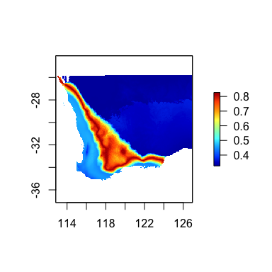
Predicted magnitude of biological change through time
Using GDM to transform environmental data rescales the individual
predictors to a common scale of biological importance. Spatially
explicit predictor data to be transformed can be a raster stack or brick
with one layer per predictor. If the model was fit with geographical
distance and raster data are provided to the transform
function, there is no need to provide x- or y-raster layers as these
will be generated automatically. However, the character names of the x-
and y-coordinates (e.g., “Long” and “Lat”) used to fit the model need to
be provided.
First we fit a new model using only the climate variables.
# fit the GDM
gdmRastMod <- gdm(data=gdmTab.rast, geo=TRUE)
We then use the gdm.transform function to rescale the
rasters.
transRasts <- gdm.transform(model=gdmRastMod, data=swBioclims)
terra::plot(transRasts, col=rgb.tables(1000))![]()
Site-pair based biological distances are difficult to visualize.
However, if the transform function is applied to rasters,
the resulting multi-dimensional biological space can be mapped to reveal
biological patterns in geographic space. Alternatively, a biplot can be
used to depict where sites fall relative to each other in biological
space and therefore how sites differ in predicted biological
composition. In either case, the multi-dimensional biological space can
be most effectively visualized by taking a PCA to reduce dimensionality
and assigning the first three components to an RGB color palette. In the
resulting map, color similarity corresponds to the similarity of
expected plant species composition (in other words, cells with similar
colors are expected to contain similar plant communities).
# Perform the principle components analysis on the gdm transformed rasters
pcaSamp <- terra::prcomp(transRasts, maxcell = 5e5)

# Predict the first three principle components for every cell in the rasters
# note the use of the 'index' argument
pcaRast <- terra::predict(transRasts, pcaSamp, index=1:3)

# Stretch the PCA rasters to make full use of the colour spectrum
pcaRast <- terra::stretch(pcaRast)

# Plot the three PCA rasters simultaneously, each representing a different colour
#  (red, green, blue)
terra::plotRGB(pcaRast, r=1, g=2, b=3)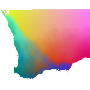
Predicted spatial variation in plant species composition. Colors represent gradients in species composition derived from transformed environmental predictors. Locations with similar colors are expected to contain similar plant communities.