
![]()
![]()

![]()
gaussplotR provides functions to fit two-dimensional
Gaussian functions, predict values from such functions, and produce
plots of predicted data.
You can install gaussplotR from CRAN via:
install.packages("gaussplotR")Or to get the latest (developmental) version through GitHub, use:
devtools::install_github("vbaliga/gaussplotR")The function fit_gaussian_2D() is the workhorse of
gaussplotR. It uses stats::nls() to find the
best-fitting parameters of a 2D-Gaussian fit to supplied data based on
one of three formula choices. The function
autofit_gaussian_2D() can be used to automatically figure
out the best formula choice and arrive at the best-fitting
parameters.
The predict_gaussian_2D() function can then be used to
predict values from the Gaussian over a supplied grid of X- and Y-values
(generated here via expand.grid()). This is useful if the
original data is relatively sparse and interpolation of values is
desired.
Plotting can then be achieved via ggplot_gaussian_2D(),
but note that the data.frame created by
predict_gaussian_2D() can be supplied to other plotting
frameworks such as lattice::levelplot(). A 3D plot can also
be produced via rgl_gaussian_2D() (not shown here).
library(gaussplotR)

## Load the sample data set
data(gaussplot_sample_data)

## The raw data we'd like to use are in columns 1:3
samp_dat <-
  gaussplot_sample_data[,1:3]


#### Example 1: Unconstrained elliptical ####
## This fits an unconstrained elliptical by default
gauss_fit_ue <-
  fit_gaussian_2D(samp_dat)

## Generate a grid of X- and Y- values on which to predict
grid <-
  expand.grid(X_values = seq(from = -5, to = 0, by = 0.1),
              Y_values = seq(from = -1, to = 4, by = 0.1))

## Predict the values using predict_gaussian_2D
gauss_data_ue <-
  predict_gaussian_2D(
    fit_object = gauss_fit_ue,
    X_values = grid$X_values,
    Y_values = grid$Y_values,
  )

## Plot via ggplot2 and metR
library(ggplot2); library(metR)
#> Warning: package 'ggplot2' was built under R version 4.0.5
#> Warning: package 'metR' was built under R version 4.0.5
ggplot_gaussian_2D(gauss_data_ue)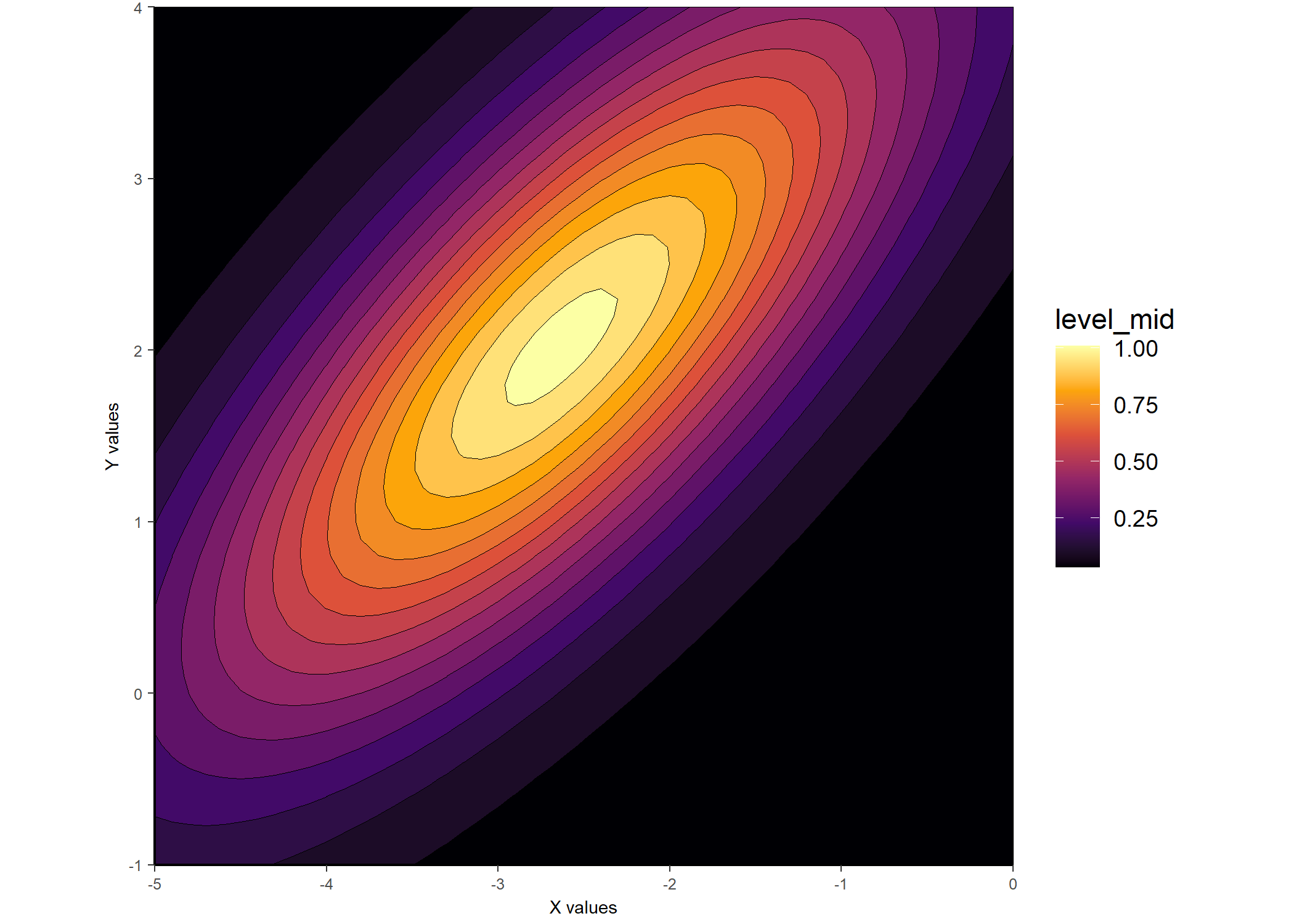
## And another example plot via lattice::levelplot()
library(lattice)
lattice::levelplot(
  predicted_values ~ X_values * Y_values,
  data = gauss_data_ue,
  col.regions = colorRampPalette(
    c("white", "blue")
    )(100),
  asp = 1
)
#### Example 2: Constrained elliptical_log ####
## This fits a constrained elliptical, as in Priebe et al. 2003
gauss_fit_cel <-
  fit_gaussian_2D(
    samp_dat,
    method = "elliptical_log",
    constrain_orientation = -1
  )

## Generate a grid of x- and y- values on which to predict
grid <-
  expand.grid(X_values = seq(from = -5, to = 0, by = 0.1),
              Y_values = seq(from = -1, to = 4, by = 0.1))

## Predict the values using predict_gaussian_2D
gauss_data_cel <-
  predict_gaussian_2D(
    fit_object = gauss_fit_cel,
    X_values = grid$X_values,
    Y_values = grid$Y_values,
  )

## Plot via ggplot2 and metR
ggplot_gaussian_2D(gauss_data_cel)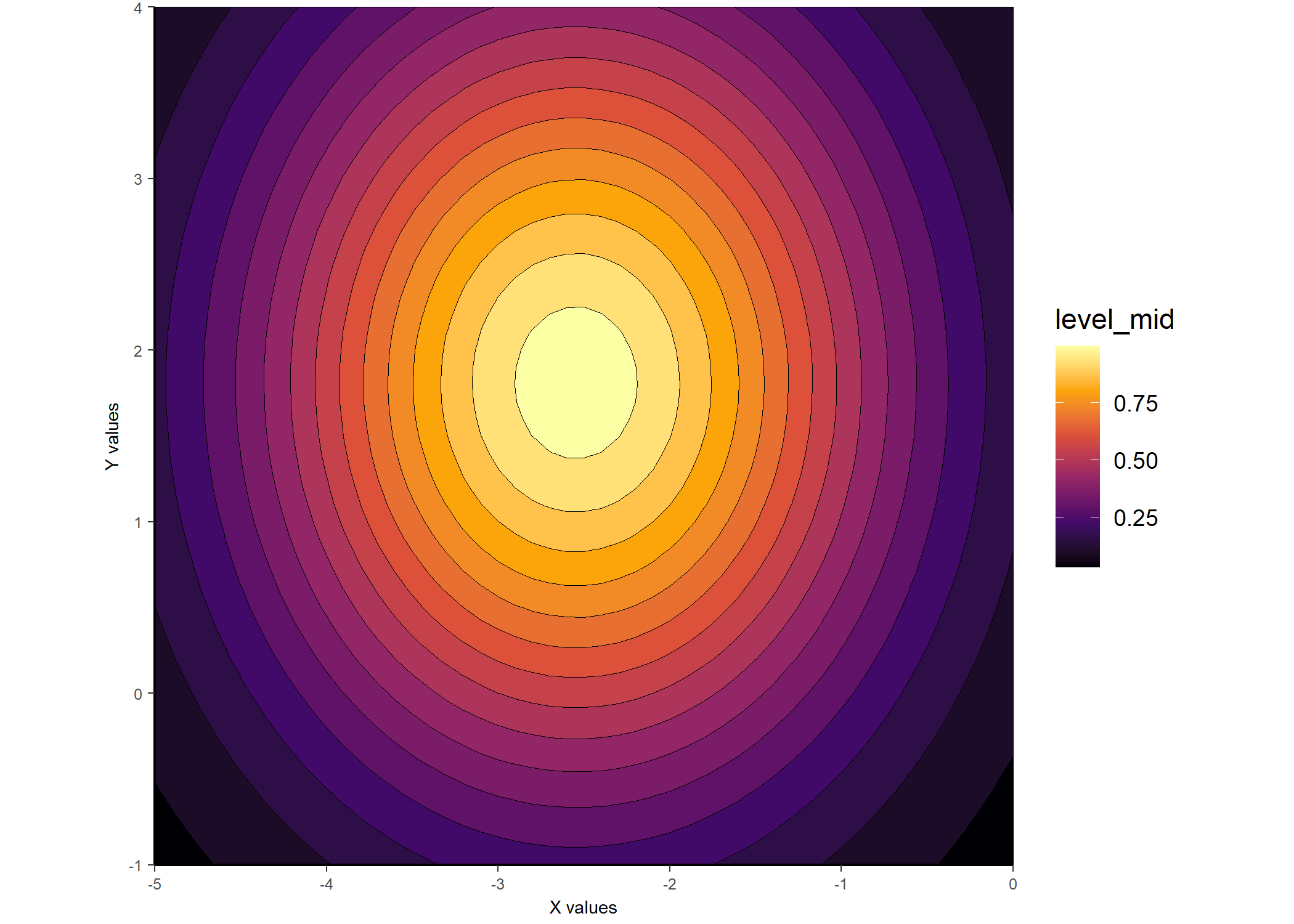
Should you be interested in having gaussplotR try to
automatically determine the best choice of method for
fit_gaussian_2D(), the autofit_gaussian_2D()
function can come in handy. The default is to select the
method that produces a fit with the lowest
rmse, but other choices include rss and
AIC.
## Use autofit_gaussian_2D() to automatically decide the best
## model to use
gauss_auto <-
  autofit_gaussian_2D(
    samp_dat,
    comparison_method = "rmse",
    simplify = TRUE
    )

## The output has the same components as `fit_gaussian_2D()`
## but for the automatically-selected best-fitting method only:
summary(gauss_auto)
#> Model coefficients
#>   A_o   Amp theta X_peak Y_peak    a    b
#>  0.83 32.25  3.58  -2.64   2.02 0.91 0.96
#> Model error stats
#>     rss rmse deviance AIC
#>  156.23 2.08   156.23 171
#> Fitting methods
#>          method       amplitude     orientation
#> "elliptical" "unconstrained" "unconstrained"Feedback on bugs, improvements, and/or feature requests are all welcome. Please see the Issues templates on GitHub to make a bug fix request or feature request.
To contribute code via a pull request, please consult the Contributing Guide first.
Baliga, VB. 2021. gaussplotR: Fit, predict, and plot 2D-Gaussians in R. Journal of Open Source Software, 6(60), 3074. https://doi.org/10.21105/joss.03074
GPL (>= 3) + file LICENSE
🐢