README

extrememix implements Bayesian estimation of extreme value mixture models, estimating the threshold over which a Generalized Pareto distribution can be assumed as well as high quantiles and other measures of interest in extreme value theory.

Installation

# install.packages("devtools")
#devtools::install_github("manueleleonelli/extrememix")

library(extrememix)
library(ggplot2)

An applied analysis

We consider the rainfall dataset reporting the monthly maxima daily rainfall (in mm) recorded at the Retiro station in the city of Madrid between 1985 and 2020. The data consists of 414 monthly maxima since 18 months were discarded in which no rain was observed.

data("rainfall")
ggplot(data = data.frame(rainfall), aes(x=rainfall)) +
  geom_histogram(binwidth = 2*length(rainfall)^(-1/3)*IQR(rainfall), colour="black", fill="white") + theme_bw()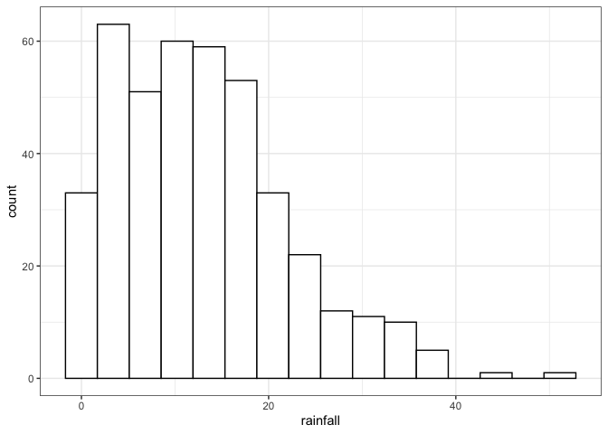

The data histogram shows that the maximum rainfall observed in a day is around 50mm. Although there are some extreme observations, the distribution appears to be right-bounded.

We start our analysis fitting the GGPD model (gamma bulk/GPD tail) using the function fggpd. We specify the number of iterations, the burn-in and the thinning via the options it, burn and thin, respectively. The prior distribution, the starting values and the variances of the proposal distributions are automatically chosen, but these can be set by the user (see below).

rainfall_ggpd <- fggpd(rainfall, it = 50000, burn = 10000, thin = 40)
rainfall_ggpd

The print method for the object model1 gives us an overview of the estimation process, stating the model fitted, its log-likelihood, the posterior estimate of the shape parameter \(\xi\) of the GPD and the probability that the distribution is right-unbounded. Additional details can be gathered using the summary function.

summary(rainfall_ggpd)
#>       estimate lower_ci upper_ci
#> xi       -0.14    -0.27     0.05
#> sigma     8.83     6.86    11.80
#> u        13.97     9.05    14.88
#> mu       16.33    14.35    20.40
#> eta       1.16     0.96     1.36

The summary reports the posterior estimates as well as 95% posterior credibility intervals of the models’ parameters. The threshold is estimated at 12.88 and the GPD is therefore estimated over a proportion of the data equal to 0.4541063.

extrememix includes the function check_convergence which reports the traceplot and the auto-correlation plot for the estimated 0.99 quantile. It can be used as a quick check to ensure convergence of the estimation algorithm. Other R packages can be used for more in-depth analyses. According to the output, the estimation of the quantile is stable and therefore it is likely that the chain reached convergence.

check_convergence(rainfall_ggpd)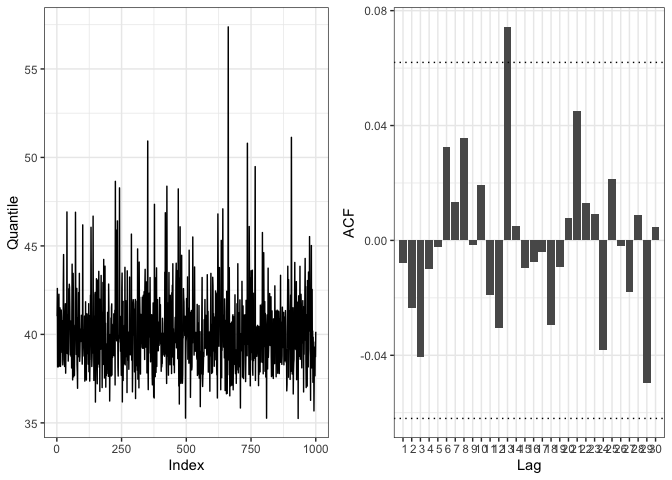

As an alternative model we consider the MGPD (mixture of gammas bulk/GPD tail) with 2 mixture components. It can be fitted using the function fmgpd, which needs as input also the number of components k. In this case we fully specify the model and the estimation procedure by also giving the starting values, the variances and the prior distribution.

The starting values can be set creating a list with entries xi, sigma, u, mu, eta and w. The proposal variances can be set creating a list with entries xi, sigma, u, mu and w (for each mixture component the parameters \(\mu\) and \(\eta\) are sampled jointly). The prior distribution can be set creating a list with entries u (a vector with the mean and standard deviation of the prior normal distribution for \(u\)), mu_mu (a vector with the prior means of the Gamma distributions for \(\mu\)), mu_eta (a vector with the prior shapes of the Gamma distributions for \(\mu\)), eta_mu (a vector with the prior means of the Gamma distributions for \(\eta\)) and eta_eta (a vector with the prior shapes of the Gamma distributions for \(\eta\)).

start <- list(xi = 0.2, sigma = 5, u = quantile(rainfall,0.9), 
              mu = c(4,10), eta = c(1,4), w = c(0.5,0.5))
var <- list(xi = 0.001, sigma = 1, u = 2, mu = c(0.1,0.1), w = 0.1)
prior <- list(u = c(22,5), mu_mu = c(4,16), mu_eta = c(0.001,0.001),
              eta_mu = c(1,4), eta_eta = c(0.001,0.001))
rainfall_mgpd <- fmgpd(rainfall, k =2, it = 50000, burn = 10000, thin = 40,
                start = start, var = var, prior = prior)

The summary below shows that an MGPD model is not actually required since the estimate of the weight of one of the two components is zero.

rainfall_mgpd
#> EVMM with 2 Mixtures of Gamma bulk. LogLik -1441.789 
#> xi estimated as  -0.1348735 
#> Probability of unbounded distribution  0.05894106
summary(rainfall_mgpd)
#>       estimate lower_ci upper_ci
#> xi       -0.13    -0.26     0.04
#> sigma     8.70     6.82    11.96
#> u        13.97     9.10    14.95
#> mu1       0.00     0.00     0.00
#> mu2      16.30    14.19    18.87
#> eta1      0.00     0.00     0.00
#> eta2      1.16     0.98     1.34
#> w1        0.00     0.00     0.00
#> w2        1.00     1.00     1.00

Let’s anyway check the convergence of the algorithm to ensure the estimation process went ok.

check_convergence(rainfall_mgpd)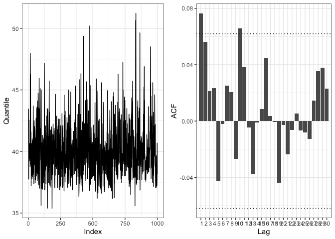

Since the MGPD model has one weight equal to zero, a GGPD is recommended. We can anyway check that this is the case using model selection criteria. extrememix implements the AIC, AICc, BIC, DIC and WAIC criteria in the equally-named functions.

rbind(c(BIC(rainfall_ggpd),BIC(rainfall_mgpd)),c(DIC(rainfall_ggpd),DIC(rainfall_mgpd)),c(WAIC(rainfall_ggpd),WAIC(rainfall_mgpd)))
#>          [,1]     [,2]
#> [1,] 2913.918 2931.784
#> [2,] 2891.035 2892.770
#> [3,] 2897.241 2896.992

For simplicity, here we considered three model selection criteria. BIC, DIC and WAIC all favor the GGPD. As already noticed in the literature, the use of WAIC is recommended and indeed it selects the GGPD model.

We therefore next investigate the use of the GGPD model to assess rainfall in the city of Madrid. The plot method gives an overview of the model reporting the histogram of the distributions of \(\xi\) and \(\sigma\), a plot of the quantiles and a plot of the predictive distribution.

plot(rainfall_ggpd)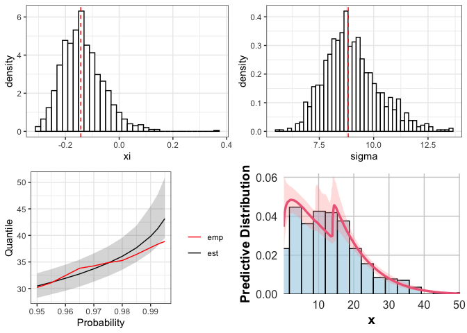

The predictive distribution can be further obtained using the function pred. The plot shows that the model gives a faithful description of the tail of the data.

pred(rainfall_ggpd)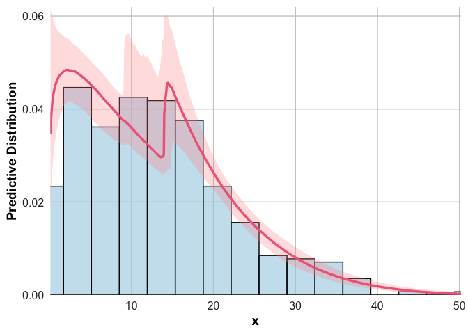

In extreme value analysis there are many measures that are used to quantify risk: quantiles (implemented in quant), return levels (in return_level), Value-at-Risk (in VaR), Expected shortfall (in ES) and Tail VaR (in TVaR). For instance here we compute the return levels, i.e. the value that is expected to be equaled or exceeded on average once every interval of time (T).

return_level(rainfall_ggpd)
#>       Level estimate lower_ci upper_ci empirical
#>  [1,]    20    30.47    28.24    32.87     30.20
#>  [2,]    25    31.93    29.58    34.49     32.44
#>  [3,]    30    33.05    30.65    35.84     34.05
#>  [4,]    40    34.79    32.33    37.92     34.87
#>  [5,]    50    36.06    33.52    39.57     35.27
#>  [6,]    60    37.09    34.50    40.88     35.80
#>  [7,]    70    37.93    35.23    42.33     36.65
#>  [8,]    80    38.64    35.84    43.68     37.02
#>  [9,]    90    39.26    36.37    44.65     37.39
#> [10,]   100    39.83    36.79    45.50     37.71
#> [11,]   150    41.79    38.46    48.61     38.52
#> [12,]   200    43.15    39.53    50.89     38.87
#> [13,]   250    44.17    40.35    52.62     41.13
plot(return_level(rainfall_ggpd))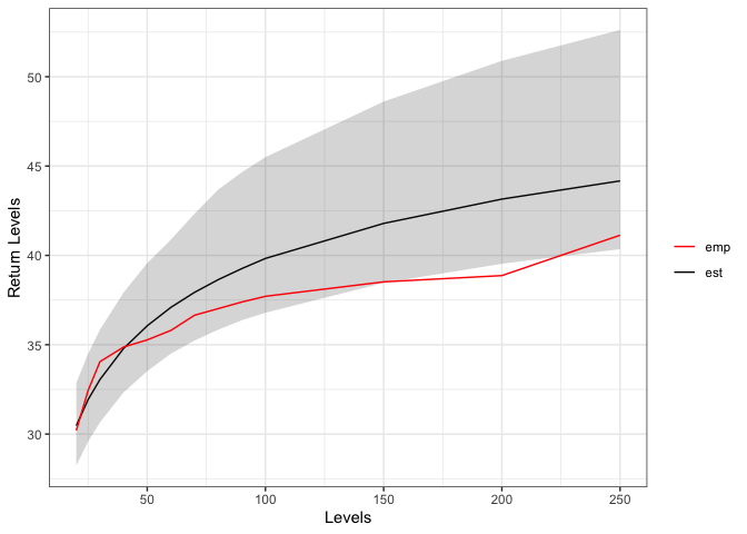

From the output we can see that we expect a rainfall of 30.42 mms to be equaled or exceeded every 20 months. The width of the credibility intervals can be chosen with the cred input and the values at which to compute the return levels can be chosen with values.

As a different measure, we consider next the expected shortfall, defined as the expected value in the q% of the worst cases. For instance, the code below computes the 1% expected shortfall.

ES(rainfall_ggpd, values = 1)
#>      ES_Level estimate lower_ci upper_ci empirical
#> [1,]        1    44.26    40.35    53.45     42.12
plot(ES(rainfall_ggpd, values = 1))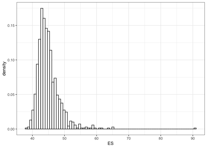

In other words, conditional on observing a value above the 0.99 quantile, the expected rainfall is equal to 44.46mms.

Since we selected a unique values the plotting method reports the posterior histogram of the estimated quantity.

To conclude the analysis, we can further estimate what is the largest possible rainfall that could ever be observed in the city of Madrid, since we observed that \(\xi\) was often estimated as negative. This can be done with the function upper_bound.

upper_bound(rainfall_ggpd)
#> Probability of unbounded distribution:  0.052 
#> Estimated upper bound at  74.07  with probability  0.948 
#>  Credibility interval at  0.95 %: ( 53.79 , 321.48 )
plot(upper_bound(rainfall_ggpd), xlim = c(20,400))
#> Upper Bound, with probability  0.948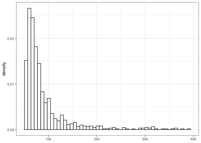

The maximum rainfall that could be observed in Madrid is estimated as 74.07. Furthermore, since in the posterior sample there are some values of \(\xi\) which are positive, we have a non-zero probability that the distribution is right-unbounded. The limits of the histogram are set with the input xlim.