The package supports shelf life estimation for chemically derived medicines, either following the standard method proposed by the International Council for Harmonisation (ICH), in quality guideline Q1E Evaluation of Stability Data or following the worst-case scenario consideration (what-if analysis) described in the Australian Regulatory Guidelines for Prescription Medicines (ARGPM), guidance on Stability testing for prescription medicines.
A stable version of expirest can be installed from CRAN:
The development version is available from GitHub by:
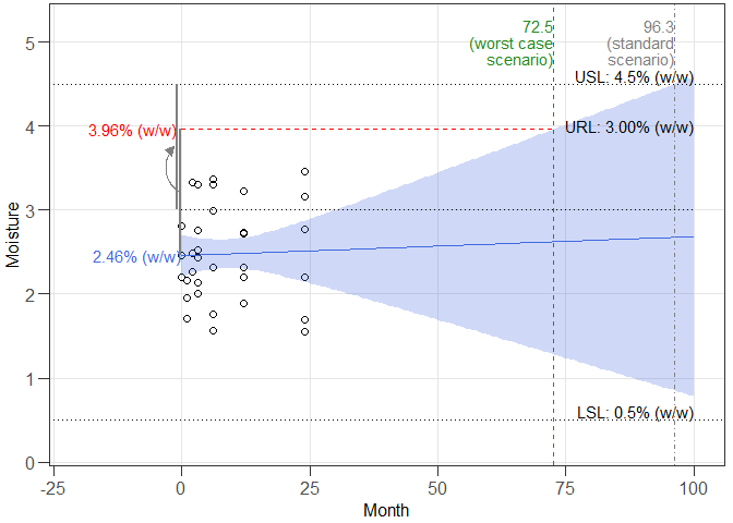
This is a basic example which shows you how to solve a common problem using a data set containing the moisture stability data (% (w/w)) of three batches obtained over a 24 months period of a drug product. A total of n = 33 independent measurements are available (corresponding to data shown in Table XIII in LeBlond et al. (2011).
library(expirest)

# Data frame
str(exp3)
#> 'data.frame':    33 obs. of  3 variables:
#>  $ Batch   : Factor w/ 3 levels "b1","b2","b3": 1 1 1 1 1 1 1 1 1 1 ...
#>  $ Month   : num  0 1 2 3 3 6 6 12 12 24 ...
#>  $ Moisture: num  2.2 1.7 3.32 2.76 2.43 ...

# Perform what-if shelf life estimation (wisle) and print a summary
res1 <- expirest_wisle(
      data = exp3, response_vbl = "Moisture", time_vbl = "Month",
      batch_vbl = "Batch", rl = 3.00, rl_sf = 3, sl = c(0.5, 4.5),
      sl_sf = c(1, 2), srch_range = c(0, 500), alpha = 0.05,
      alpha_pool = 0.25, xform = c("no", "no"), shift = c(0, 0),
      sf_option = "tight", ivl = "confidence", ivl_type = "one.sided",
      ivl_side = "upper")

class(res1)
#> [1] "expirest_wisle"
summary(res1)
#>
#> Summary of shelf life estimation following the ARGPM
#>   guidance "Stability testing for prescription medicines"
#>
#> The best model accepted at a significance level of 0.25 has
#>  Common intercepts and Common slopes (acronym: cics).
#>
#> Worst case intercept and batch:
#>   RL Batch Intercept
#> 1  3    NA  2.456782
#>
#> Estimated shelf lives for the cics model:
#>    SL RL    wisle     osle
#> 1 4.5  3 72.50545 96.30552
#>
#> Abbreviations:
#>   ARGPM: Australian Regulatory Guidelines for Prescription Medicines;
#>   ICH: International Council for Harmonisation;
#>   osle: Ordinary shelf life estimation (i.e. following the ICH guidance);
#>   RL: Release Limit;
#>   SL: Specification Limit;
#>   wisle: What-if (approach for) shelf life estimation (see ARGPM guidance).

# Prepare graphical representation
ggres1 <- plot_expirest_wisle(
      model = res1, rl_index = 1, response_vbl_unit = "% (w/w)",
      x_range = NULL, y_range = c(0.2, 5.2), scenario = "standard",
      mtbs = "verified", plot_option = "full", ci_app = "ribbon")
class(ggres1)
#> [1] "plot_expirest_wisle"
plot(ggres1)
The model type in Example 1 was common intercept / common slope (cics). The model type in this example is different intercept / different slope (dids). A data set containing the potency stability data (in % of label claim (LC)) of five batches of a drug product obtained over a 24 months period is used. A total of n = 53 independent measurements are available (corresponding to data shown in Tables IV, VI and VIII in LeBlond et al. (2011).
# Data frame
str(exp1)
#> 'data.frame':    53 obs. of  3 variables:
#>  $ Batch  : Factor w/ 6 levels "b2","b3","b4",..: 1 1 1 1 1 1 1 1 1 1 ...
#>  $ Month  : num  0 1 3 3 6 6 12 12 24 24 ...
#>  $ Potency: num  101 101.3 99.8 99.2 99.5 ...

# Perform what-if shelf life estimation (wisle) and print a summary
res2_1 <- expirest_wisle(
      data = exp1[exp1$Batch %in% c("b4", "b5", "b8"), ],
      response_vbl = "Potency", time_vbl = "Month", batch_vbl = "Batch",
      rl = c(98.0, 98.5, 99.0), rl_sf = rep(2, 3), sl = 95, sl_sf = 2,
      srch_range = c(0, 500), alpha = 0.05, alpha_pool = 0.25,
      xform = c("no", "no"), shift = c(0, 0), sf_option = "tight",
      ivl = "confidence", ivl_type = "one.sided", ivl_side = "lower")

summary(res2_1)
#>
#> Summary of shelf life estimation following the ARGPM
#>   guidance "Stability testing for prescription medicines"
#>
#> The best model accepted at a significance level of 0.25 has
#>  Different intercepts and Different slopes (acronym: dids).
#>
#> Worst case intercepts and batches:
#>     RL Batch Intercept
#> 1 98.0    b8  101.2594
#> 2 98.5    b8  101.2594
#> 3 99.0    b8  101.2594
#>
#> Estimated shelf lives for the dids model (for information, the results of
#>   the model fitted with pooled mean square error (pmse) are also shown:
#>   SL   RL     wisle wisle (pmse)     osle osle (pmse)
#> 1 95 98.0  7.619661     7.483223 15.84487     15.6061
#> 2 95 98.5  8.997036     8.858223 15.84487     15.6061
#> 3 95 99.0 10.303030    11.344407 15.84487     15.6061
#>
#> Abbreviations:
#>   ARGPM: Australian Regulatory Guidelines for Prescription Medicines;
#>   ICH: International Council for Harmonisation;
#>   osle: Ordinary shelf life estimation (i.e. following the ICH guidance);
#>   pmse: Pooled mean square error;
#>   RL: Release Limit;
#>   SL: Specification Limit;
#>   wisle: What-if (approach for) shelf life estimation (see ARGPM guidance).

# Prepare graphical representation
ggres2_1 <- plot_expirest_wisle(
      model = res2_1, rl_index = 2, response_vbl_unit = "%", x_range = NULL,
      y_range = c(93, 107), scenario = "standard", mtbs = "verified",
      plot_option = "full", ci_app = "ribbon")
class(ggres2_1)
#> [1] "plot_expirest_wisle"
plot(ggres2_1)
Note that if the model type is dids, then by default the results are plotted that are obtained by fitting individual regression lines to each batch. To get a plot of the dids model with pooled mean square error (pmse) instead, use the setting mtbs = "dids.pmse".
# Prepare graphical representation of the dids.pmse model
ggres2_2 <- plot_expirest_wisle(
      model = res2_1, rl_index = 2, response_vbl_unit = "%", x_range = NULL,
      y_range = c(93, 107), scenario = "standard", mtbs = "dids.pmse",
      plot_option = "full", ci_app = "ribbon")
plot(ggres2_2)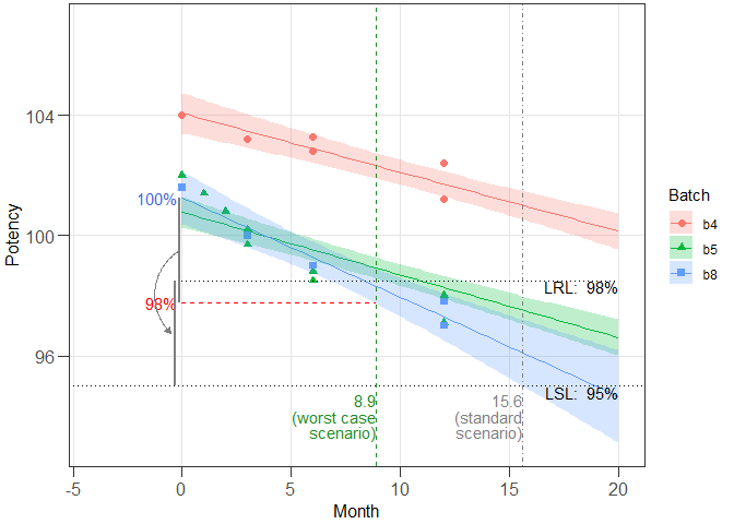
The examples above were performed with three batches. The assessment can be performed with any numbers of batches, even with just one batch. If the assessment is performed with a single batch, the results are reported as dids model while the results for all other models are NA. As an example, the following example was performed with batch b4.
# Perform what-if shelf life estimation (wisle) and print a summary
res2_2 <- expirest_wisle(
      data = exp1[exp1$Batch == "b4", ],
      response_vbl = "Potency", time_vbl = "Month", batch_vbl = "Batch",
      rl = c(98.0, 98.5, 99.0), rl_sf = rep(2, 3), sl = 95, sl_sf = 2,
      srch_range = c(0, 500), alpha = 0.05, alpha_pool = 0.25,
      xform = c("no", "no"), shift = c(0, 0), sf_option = "tight",
      ivl = "confidence", ivl_type = "one.sided", ivl_side = "lower")

summary(res2_2)
#>
#> Summary of shelf life estimation following the ARGPM
#>   guidance "Stability testing for prescription medicines"
#>
#> The best model accepted at a significance level of 0.25 has
#>  NA intercepts and NA slopes (acronym: n.a.).
#>
#> Worst case intercepts and batches:
#>     RL Batch Intercept
#> 1 98.0    b4  104.0706
#> 2 98.5    b4  104.0706
#> 3 99.0    b4  104.0706
#>
#> Estimated shelf lives for the n.a. model (for information, the results of
#>   the model fitted with pooled mean square error (pmse) are also shown:
#>   SL   RL    wisle wisle (pmse)     osle osle (pmse)
#> 1 95 98.0 13.72633           NA 40.79176          NA
#> 2 95 98.5 16.09778           NA 40.79176          NA
#> 3 95 99.0 18.40465           NA 40.79176          NA
#>
#> Abbreviations:
#>   ARGPM: Australian Regulatory Guidelines for Prescription Medicines;
#>   ICH: International Council for Harmonisation;
#>   osle: Ordinary shelf life estimation (i.e. following the ICH guidance);
#>   pmse: Pooled mean square error;
#>   RL: Release Limit;
#>   SL: Specification Limit;
#>   wisle: What-if (approach for) shelf life estimation (see ARGPM guidance).

# Prepare graphical representation
ggres2_2 <- plot_expirest_wisle(
      model = res2_2, rl_index = 2, response_vbl_unit = "%", x_range = NULL,
      y_range = c(93, 107), scenario = "standard", mtbs = "verified",
      plot_option = "full", ci_app = "ribbon")
plot(ggres2_2)
The assessments in Example 1 and Example 2 were made with the option sf_option = "tight". The parameter sf_option affects the shelf life (sl) and release limits (rl). The setting sf_option = "tight" means that of the sl and rl limits only the number of significant digits specified by the parameters rl_sf and sl_sf, respectively, are taken into account. If sf_option = "loose", then the limits are widened, i.e. four on the order of the last significant digit + 1 is added if ivl_side = "upper" or five on the order of the last significant digit + 1 is subtracted if ivl_side = "lower". For illustration, the following example reproduces Example 2 with the option sf_option = "loose".
# Perform what-if shelf life estimation (wisle) and print a summary
res3 <- expirest_wisle(
      data = exp1[exp1$Batch %in% c("b4", "b5", "b8"), ],
      response_vbl = "Potency", time_vbl = "Month", batch_vbl = "Batch",
      rl = c(98.0, 98.5, 99.0), rl_sf = rep(3, 3), sl = 95, sl_sf = 2,
      srch_range = c(0, 500), alpha = 0.05, alpha_pool = 0.25,
      xform = c("no", "no"), shift = c(0, 0), sf_option = "loose",
      ivl = "confidence", ivl_type = "one.sided", ivl_side = "lower")

summary(res3)
#>
#> Summary of shelf life estimation following the ARGPM
#>   guidance "Stability testing for prescription medicines"
#>
#> The best model accepted at a significance level of 0.25 has
#>  Different intercepts and Different slopes (acronym: dids).
#>
#> Worst case intercepts and batches:
#>     RL Batch Intercept
#> 1 98.0    b8  101.2594
#> 2 98.5    b8  101.2594
#> 3 99.0    b8  101.2594
#>
#> Estimated shelf lives for the dids model (for information, the results of
#>   the model fitted with pooled mean square error (pmse) are also shown:
#>   SL   RL     wisle wisle (pmse)    osle osle (pmse)
#> 1 95 98.0  8.863085     8.724968 17.0387    16.77679
#> 2 95 98.5 10.174754    11.221221 17.0387    16.77679
#> 3 95 99.0 11.440468    11.276686 17.0387    16.77679
#>
#> Abbreviations:
#>   ARGPM: Australian Regulatory Guidelines for Prescription Medicines;
#>   ICH: International Council for Harmonisation;
#>   osle: Ordinary shelf life estimation (i.e. following the ICH guidance);
#>   pmse: Pooled mean square error;
#>   RL: Release Limit;
#>   SL: Specification Limit;
#>   wisle: What-if (approach for) shelf life estimation (see ARGPM guidance).

# Prepare graphical representation
ggres3 <- plot_expirest_wisle(
      model = res3, rl_index = 2, response_vbl_unit = "%", x_range = NULL,
      y_range = c(93, 107), scenario = "standard", mtbs = "verified",
      plot_option = "full", ci_app = "ribbon")
plot(ggres3)
LeBlond, D., Griffith, D. and Aubuchon, K. Linear Regression 102: Stability Shelf Life Estimation Using Analysis of Covariance. J Valid Technol (2011) 17(3): 47-68.
Pius Dahinden, Tillotts Pharma AG