![]()
![]()
evabic aims to evaluate binary classifiers by specifying what is detected as true and what is actually true. It has no dependencies.
You can install evabic from CRAN using
install.packages("evabic"). Alternatively you can grab the
development version from GitHub with:
# install.packages("pak")
pak::pak("abichat/evabic")evabic provides handy functions to compute 18
different measures. Each function begins with ebc_*.
Available measures include True Positive Rate (Sensitivity or Recall), True Negative Rate (Specificity), Positive Predictive Value (Precision), False Discovery Rate, Accuracy, F1…
evabic::ebc_allmeasures
#> [1] "TP" "FP" "FN" "TN" "TPR" "TNR" "PPV" "NPV" "FNR" "FPR"
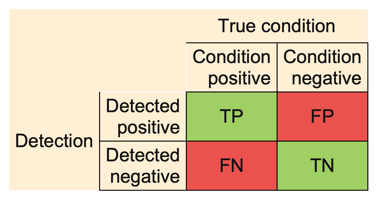
#> [11] "FDR" "FOR" "ACC" "BACC" "F1" "PLR" "NLR" "DOR"All measures are computed from the confusion matrix:
Let’s use evabic on a toy example.
library(evabic)Consider three variables X1, X2 and
X3, Y a variable predicted by this three
variables, and 4 more conditionally independent variables
X4 to X7.
set.seed(42)
X1 <- rnorm(50)
X2 <- rnorm(50)
X3 <- rnorm(50)
predictors <- paste0("X", 1:3)

df_lm <- data.frame(
  X1 = X1,
  X2 = X2,
  X3 = X3,
  X4 = X1 + X2 + X3 + rnorm(50, sd = 0.5),
  X5 = X1 + 3 * X3 + rnorm(50, sd = 0.5),
  X6 = X2 - 2 * X3 + rnorm(50, sd = 0.5),
  X7 = X1 - 0.2 * X2 + rnorm(50, sd = 2),
  Y = X1 - 0.2 * X2 + 3 * X3 + rnorm(50)
)
We use a linear regression to detect the actual predictors (do not select significant variables like this at home, it’s a bad way to do so).
model <- lm(Y ~ ., data = df_lm)
summary(model)
#>
#> Call:
#> lm(formula = Y ~ ., data = df_lm)
#>
#> Residuals:
#>      Min       1Q   Median       3Q      Max
#> -1.66504 -0.65784 -0.05977  0.51720  2.14833
#>
#> Coefficients:
#>             Estimate Std. Error t value Pr(>|t|)
#> (Intercept)  0.13537    0.14528   0.932  0.35678
#> X1           1.35385    0.44929   3.013  0.00437 **
#> X2           0.09974    0.46105   0.216  0.82977
#> X3           3.67893    1.18759   3.098  0.00347 **
#> X4          -0.22998    0.33164  -0.693  0.49183
#> X5          -0.17073    0.30744  -0.555  0.58161
#> X6          -0.04023    0.28381  -0.142  0.88795
#> X7           0.07055    0.09245   0.763  0.44966
#> ---
#> Signif. codes:  0 '***' 0.001 '**' 0.01 '*' 0.05 '.' 0.1 ' ' 1
#>
#> Residual standard error: 1.005 on 42 degrees of freedom
#> Multiple R-squared:  0.921,  Adjusted R-squared:  0.9079
#> F-statistic: 69.99 on 7 and 42 DF,  p-value: < 2.2e-16
pvalues <- summary(model)$coefficients[-1, 4]
pvalues
#>          X1          X2          X3          X4          X5          X6
#> 0.004366456 0.829771754 0.003469737 0.491828466 0.581608670 0.887948400
#>          X7
#> 0.449664443
detected_var <- names(pvalues[pvalues < 0.05])
detected_var
#> [1] "X1" "X3"
Here, we selected two predictors among the three true predictors.
Single measures are available with ebc_*()
functions.
ebc_TPR(detected = detected_var, true = predictors)
#> [1] 0.6666667
ebc_ACC(detected = detected_var, true = predictors, m = 7) # the total size of the set is 7
#> [1] 0.8571429
You can also ask for several measures in a single row summary format
with ebc_tidy().
ebc_tidy(
  detected = detected_var,
  true = predictors,
  m = 7,
  # you can use `measures = ebc_allmeasures` to compute all measures
  measures = c("TPR", "TNR", "FDR", "ACC", "BACC", "F1")
)
#>         TPR TNR FDR       ACC      BACC  F1
#> 1 0.6666667   1   0 0.8571429 0.8333333 0.8
Note that evabic also supports named logicals for
detected and true arguments, but they must be
named (see the add_names() function if needed).
pvalues < 0.05
#>    X1    X2    X3    X4    X5    X6    X7
#>  TRUE FALSE  TRUE FALSE FALSE FALSE FALSE
ebc_tidy(
  detected = pvalues < 0.05,
  true = predictors,
  m = 7,
  measures = c("TPR", "TNR", "FDR", "ACC", "BACC", "F1")
)
#>         TPR TNR FDR       ACC      BACC  F1
#> 1 0.6666667   1   0 0.8571429 0.8333333 0.8
With ebc_tidy_by_threshold(), you can ask for the
evolution of measures according to a moving threshold if you provide the
vector of p-values (or any score).
df_measures <- ebc_tidy_by_threshold(
  detection_values = pvalues,
  true = predictors,
  m = 7,
  measures = c("TPR", "FPR", "FDR", "ACC", "BACC", "F1")
)
df_measures
#>     threshold       TPR  FPR       FDR       ACC      BACC        F1
#> 1 0.003469737 0.0000000 0.00       NaN 0.5714286 0.5000000 0.0000000
#> 2 0.004366456 0.3333333 0.00 0.0000000 0.7142857 0.6666667 0.5000000
#> 3 0.449664443 0.6666667 0.00 0.0000000 0.8571429 0.8333333 0.8000000
#> 4 0.491828466 0.6666667 0.25 0.3333333 0.7142857 0.7083333 0.6666667
#> 5 0.581608670 0.6666667 0.50 0.5000000 0.5714286 0.5833333 0.5714286
#> 6 0.829771754 0.6666667 0.75 0.6000000 0.4285714 0.4583333 0.5000000
#> 7 0.887948400 1.0000000 0.75 0.5000000 0.5714286 0.6250000 0.6666667
#> 8         Inf 1.0000000 1.00 0.5714286 0.4285714 0.5000000 0.6000000
This makes it easy to plot various-threshold curves like ROC curve.
plot(
  df_measures$FPR,
  df_measures$TPR,
  type = "b",
  xlab = "FPR",
  ylab = "TPR"
)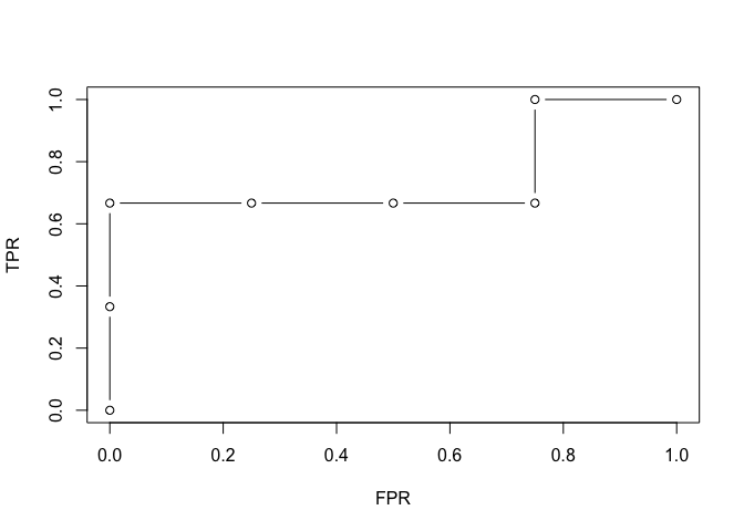
And finally, you can ask for the AUC, the area under the ROC curve.
ebc_AUC(detection_values = pvalues, true = predictors, m = 7)
#> [1] 0.75
ebc_AUC_from_measures(df_measures)
#> [1] 0.75