![]()
![]()
![]()
etrm is an R package with tools for trading and
financial risk management in energy markets. The package currently offer
tools for two main activities:
The development version can be installed from GitHub with:
devtools::install_github("sleire/etrm")The following sections provide examples using some of the synthetic data sets included in the package.
A typical characteristic of energy commodities such as electricity
and natural gas is that delivery takes place over a period in time, not
on a single date. Listed futures contracts cover standardized periods,
such as “Week”, “Month”, “Quarter”, “Season” or “Year”. The forward
curve is an essential tool for pricing non-standard OTC contracts having
any settlement period. An example of such standard energy market
contracts can be found in the package data set
powfutures130513.
#>    Include Contract      Start        End Closing
#> 1     TRUE   W21-13 2013-05-20 2013-05-26   33.65
#> 2     TRUE   W22-13 2013-05-27 2013-06-02   35.77
#> 3     TRUE   W23-13 2013-06-03 2013-06-09   36.58
#> 4     TRUE   W24-13 2013-06-10 2013-06-16   35.93
#> 5     TRUE   W25-13 2013-06-17 2013-06-23   33.14
#> 6     TRUE   W26-13 2013-06-24 2013-06-30   34.16
#> 7    FALSE  MJUN-13 2013-06-01 2013-06-30   35.35
#> 8     TRUE  MJUL-13 2013-07-01 2013-07-31   33.14
#> 9     TRUE  MAUG-13 2013-08-01 2013-08-31   35.72
#> 10    TRUE  MSEP-13 2013-09-01 2013-09-30   38.41
#> 11    TRUE  MOCT-13 2013-10-01 2013-10-31   38.81
#> 12    TRUE  MNOV-13 2013-11-01 2013-11-30   40.94
#> 13   FALSE    Q3-13 2013-07-01 2013-09-30   35.72
#> 14    TRUE    Q4-13 2013-10-01 2013-12-31   40.53
#> 15    TRUE    Q1-14 2014-01-01 2014-03-31   42.40
#> 16    TRUE    Q2-14 2014-04-01 2014-06-30   33.39
#> 17    TRUE    Q3-14 2014-07-01 2014-09-30   31.78
#> 18    TRUE    Q4-14 2014-10-01 2014-12-31   38.25
#> 19    TRUE    Q1-15 2015-01-01 2015-03-31   40.73
#> 20    TRUE    Q2-15 2015-04-01 2015-06-30   32.64
#> 21    TRUE    Q3-15 2015-07-01 2015-09-30   30.87
#> 22    TRUE    Q4-15 2015-10-01 2015-12-31   37.22
#> 23   FALSE   CAL-14 2014-01-01 2014-12-31   36.43
#> 24   FALSE   CAL-15 2015-01-01 2015-12-31   35.12
#> 25    TRUE   CAL-16 2016-01-01 2016-12-31   34.10
#> 26   FALSE   CAL-17 2017-01-01 2017-12-31   35.22
#> 27   FALSE   CAL-18 2018-01-01 2018-12-31   36.36
#> 28   FALSE   CAL-19 2019-01-01 2019-12-31   37.44
#> 29   FALSE   CAL-20 2020-01-01 2020-12-31   38.58
#> 30   FALSE   CAL-21 2021-01-01 2021-12-31   39.73
#> 31   FALSE   CAL-22 2022-01-01 2022-12-31   40.93
#> 32   FALSE   CAL-23 2023-01-01 2023-12-31   42.15
The function msfc() will create an instance of the S4
class MSFC with generic methods plot(),
summary() and show(). In addition to the
arguments from the list of contracts, the user may also provide a prior
function to the calculation. This is relevant for markets with strong
seasonality, such as power markets. The default value is
prior = 0, but the user can provide any vector expressing a
belief regarding the market to be combined with the observed prices. In
the example below we have used a simple seasonal prior from the package
powpriors130513 data set.
fwd_fut_wpri <- msfc(tdate = as.Date("2013-05-13"),          # trading date
                     include = powfutures130513$Include,     # vector with TRUE/FALSE, include contract?
                     contract = powfutures130513$Contract,   # vector with contract names
                     sdate = powfutures130513$Start,         # vector with contract start dates
                     edate = powfutures130513$End,           # vector with contract end dates
                     f = powfutures130513$Closing,           # vector with contract closing prices
                     prior = powpriors130513$mod.prior       # prior function
                     )

plot(fwd_fut_wpri, legend = "", title = "MSFC with prior for power futures 2013-05-13")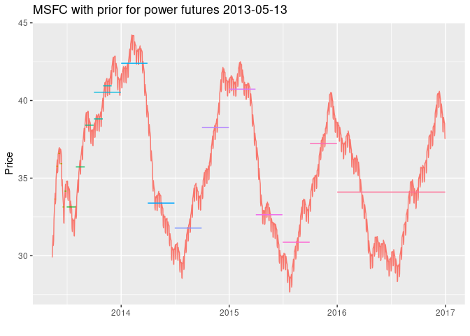
The forward curve is calculated with the function
f(t) = λ(t) + ϵ(t)
where λ(t) is the prior supplied by the user and
ϵ(t) is an adjustment function taking the observed
prices into account. The msfc() function finds the
smoothest possible adjustment function by minimizing the mean squared
value of a spline function, while ensuring that the average value of the
curve f(t) is equal to contract prices used in the
calculation for the respective time intervals. The number of polynomials
used in the spline along with head(prior) and computed
prices based on the curve are available with the summary()
method:
summary(fwd_fut_wpri)
#> $Description
#> [1] "MSFC of length 1329 built with 41 polynomials at trade date 2013-05-13"
#>
#> $PriorFunc
#> [1] 30.10842 30.16396 30.19572 30.16144 29.06268 28.93272
#>
#> $BenchSheet
#>    Include Contract       From         To Price  Comp
#> 1     TRUE   W21-13 2013-05-20 2013-05-26 33.65 33.65
#> 2     TRUE   W22-13 2013-05-27 2013-06-02 35.77 35.77
#> 3     TRUE   W23-13 2013-06-03 2013-06-09 36.58 36.58
#> 4     TRUE   W24-13 2013-06-10 2013-06-16 35.93 35.93
#> 5     TRUE   W25-13 2013-06-17 2013-06-23 33.14 33.14
#> 6     TRUE   W26-13 2013-06-24 2013-06-30 34.16 34.16
#> 8     TRUE  MJUL-13 2013-07-01 2013-07-31 33.14 33.14
#> 9     TRUE  MAUG-13 2013-08-01 2013-08-31 35.72 35.72
#> 10    TRUE  MSEP-13 2013-09-01 2013-09-30 38.41 38.41
#> 11    TRUE  MOCT-13 2013-10-01 2013-10-31 38.81 38.81
#> 12    TRUE  MNOV-13 2013-11-01 2013-11-30 40.94 40.94
#> 14    TRUE    Q4-13 2013-10-01 2013-12-31 40.53 40.53
#> 15    TRUE    Q1-14 2014-01-01 2014-03-31 42.40 42.40
#> 16    TRUE    Q2-14 2014-04-01 2014-06-30 33.39 33.39
#> 17    TRUE    Q3-14 2014-07-01 2014-09-30 31.78 31.78
#> 18    TRUE    Q4-14 2014-10-01 2014-12-31 38.25 38.25
#> 19    TRUE    Q1-15 2015-01-01 2015-03-31 40.73 40.73
#> 20    TRUE    Q2-15 2015-04-01 2015-06-30 32.64 32.64
#> 21    TRUE    Q3-15 2015-07-01 2015-09-30 30.87 30.87
#> 22    TRUE    Q4-15 2015-10-01 2015-12-31 37.22 37.22
#> 25    TRUE   CAL-16 2016-01-01 2016-12-31 34.10 34.10
The calculation without prior function, for comparison:
fwd_fut_npri <- msfc(tdate = as.Date("2013-05-13"),         # trading date
                     include = powfutures130513$Include,    # vector with TRUE/FALSE, include contract?
                     contract = powfutures130513$Contract,  # vector with contract names
                     sdate = powfutures130513$Start,        # vector with contract start dates
                     edate = powfutures130513$End,          # vector with contract end dates
                     f = powfutures130513$Closing,          # vector with contract closing prices
                     prior = 0                              # no prior function
                     )

plot(fwd_fut_npri, legend = "", title = "MSFC excluding prior for power futures 2013-05-13")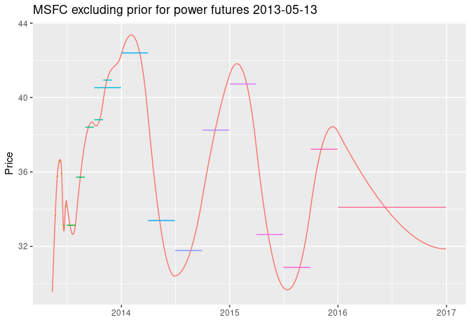
The daily forward curve values can be found along with the prior
function and contracts used in the calculation with the
show() method. An instance of MSFC is a rather
rich object, and further details regarding the calculation, spline
coefficients, etc. can be found in the slots:
slotNames(fwd_fut_wpri)
#> [1] "Name"        "TradeDate"   "BenchSheet"  "Polynomials" "PriorFunc"
#> [6] "Results" "SplineCoef" "KnotPoints" "CalcDat"Futures trading strategies for price risk management, for commercial hedgers with long or short exposure. All models below aim to achieve a favorable unit price for the energy portfolio, while preventing it from breaching a pre defined cap (floor).
The functions
cppi() - Constant Proportion Portfolio Insurancedppi() - Dynamic Proportion Portfolio Insuranceobpi() - Option Based Portfolio Insuranceshpi() - Step Hedge Portfolio Insuranceslpi() - Stop Loss Portfolio Insuranceimplement alternative approaches to achieve this goal. They return S4
objects of type CPPI, DPPI, OBPI,
SHPI and SLPI respectively, with methods
plot(), summary() and show().
In our example, we will consider the CAL-06 contract in the synthetic
powcal data set, and start trading 500 days prior to the
contract expiry. For the OBPIstrategy presented below, the
target price is calculated as an expected cap (floor) given by the
option premium-adjusted strike price selected for the delta hedging
scheme within a standard Black-76 option pricing framework. The default
strike price is set at-the-money. The user may express a view regarding
future market development by deviating from this level.
cal06_obpi_b <- obpi(q = 30,               # volume 30 MW (buyer)
                     tdate = dat06$Date,   # vector with trading days until expiry
                     f = dat06$CAL06,      # vector with futures price
                     k = dat06$CAL06[1],   # default option strike price at-the-money
                     vol = 0.2,            # annualized volatility, for the Black-76 delta hedging
                     r = 0,                # default assumed risk free rate of interest
                     tdays = 250,          # assumed trading days per year
                     daysleft = 500,       # number of days to expiry
                     tcost = 0,            # transaction cost
                     int = TRUE            # integer restriction, smallest transacted unit = 1
                   )

plot(cal06_obpi_b, legend = "bottom", title = "OBPI strategy buyer CAL-06")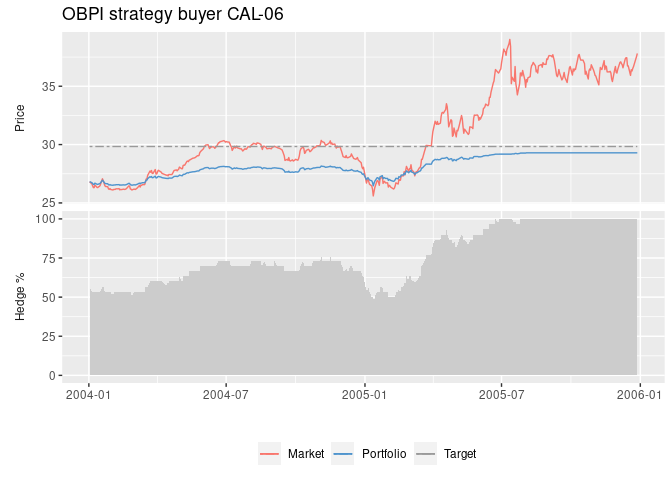
The summary() method:
summary(cal06_obpi_b)
#> $Description
#> [1] "Hedging strategy of type OBPI and length 500"
#>
#> $Volume
#> [1] 30
#>
#> $Target
#> [1] 29.83626
#>
#> $ChurnRate
#> [1] 4.333333
#>
#> $Stats
#>       Market Trade Exposed Position     Hedge   Target Portfolio
#> First  26.82    17      13       17 0.5666667 29.83626  26.82000
#> Max    39.01    17      17       30 1.0000000 29.83626  29.29433
#> Min    25.60    -3       0       13 0.4333333 29.83626  26.46833
#> Last   37.81     0       0       30 1.0000000 29.83626  29.29433
The show()method provide details regarding daily values
for market price, transactions, exposed volume, futures contract
position, the target price and the calculated portfolio price. Further
details for a specific instance of a trading strategy can be found in
the slots, see for example:
slotNames(cal06_obpi_b)
#>  [1] "StrikePrice"  "AnnVol"       "InterestRate" "TradingDays"  "Name"
#>  [6] "Volume"       "TargetPrice"  "TransCost"    "TradeisInt"   "Results"
The CAL-06 OBPI strategy from a sellers point of view:
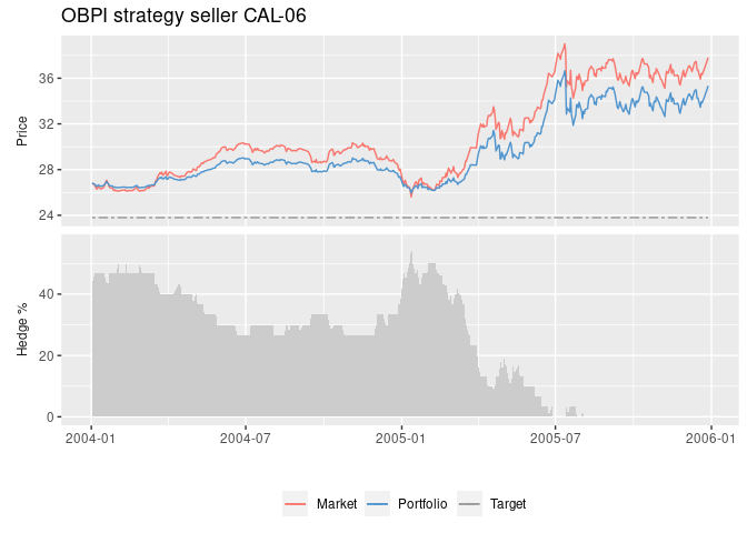
cal06_obpi_s <- obpi(q = - 30,             # volume -30 MW (seller)
                     tdate = dat06$Date,   # vector with trading days until expiry
                     f = dat06$CAL06,      # vector with futures price
                     k = dat06$CAL06[1],   # default option strike price at-the-money
                     vol = 0.2,            # annualized volatility, for the Black-76 delta hedging
                     r = 0,                # default assumed risk free rate of interest
                     tdays = 250,          # assumed trading days per year
                     daysleft = 500,       # number of days to expiry
                     tcost = 0,            # transaction cost
                     int = TRUE            # integer restriction, smallest transacted unit = 1
                   )

plot(cal06_obpi_s, legend = "bottom", title = "OBPI strategy seller CAL-06")