![]()
The goal of crimedata is to access police-recorded crime data from large US cities using the Crime Open Database (CODE), a service that provides these data in a convenient format for analysis. All the data are available to use for free as long as you acknowledge the source of the data.
The function get_crime_data() returns a tidy data tibble or simple features (SF)
object of crime data with each row representing a single crime. The
data provided for each offense includes the offense type, approximate
offense location and date/time. More fields are available for some
records, depending on what data have been released by each city. For
most cities, data are available from 2010 onward, with some available
back to 2007. Use list_crime_data() to see which years are
available for which cities.
More detail about what data are available, how they were constructed and the meanings of the different categories can be found on the CODE project website. Further detail is available in the paper Studying Crime and Place with the Crime Open Database.
You can install the crimedata package with:
install.packages("crimedata")You can install the latest development version of the crimedata package from GitHub with:
# install.packages("remotes")
remotes::install_github("mpjashby/crimedata")Data can be downloaded by year and by city. By default (i.e. if no arguments are specified) a 1% sample of data for all cities for the most recent available year is returned.
library(crimedata)

crime_data <- get_crime_data()
The data are in a tidy format, so can be quickly manipulated using dplyr verbs. For example, to analyze two years of personal robberies in Chicago and Detroit, you can run:
suppressPackageStartupMessages(library(tidyverse))

personal_robberies <- get_crime_data(
  years = 2009:2010,
  cities = c("Chicago", "Detroit"),
  type = "core",
  quiet = TRUE
) %>%
  filter(offense_type == "personal robbery")
You can alternatively get a simple features
(SF) point object with the correct co-ordinates and co-ordinate
reference system (CRS) specified by setting the argument
output = "sf". This can be used, for example, to quickly
plot the data.
suppressPackageStartupMessages(library(lubridate))

get_crime_data(
  cities = "Fort Worth",
  years = 2014:2017,
  type = "core",
  quiet = TRUE,
  output = "sf"
) %>%
  filter(offense_group == "homicide offenses") %>%
  mutate(offense_year = year(date_single)) %>%
  ggplot() +
  geom_sf() +
  facet_wrap(vars(offense_year), nrow = 1)
#> Warning: Unknown columns: `location_type`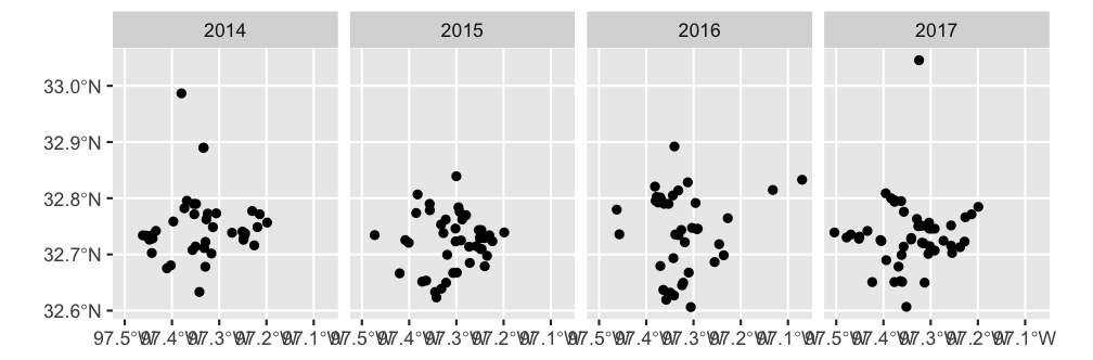
plot of chunk crimedata_sf_example
The package includes two datasets. homicides15 contains
records of 1,922 recorded homicides in nine US cities in 2015.
nycvehiclethefts contains records of 35,746 thefts of motor
vehicles in New York City from 2014 to 2017. These may be particularly
useful for teaching purposes.