
![]()
chemCal is an R package providing some basic functions for conveniently working with linear calibration curves with one explanatory variable.
From within R, get the official chemCal release using
install.packages("chemCal")chemCal works with univariate linear models of class lm.
Working with one of the datasets coming with chemCal, we can produce a
calibration plot using the calplot function:
library(chemCal)
m0 <- lm(y ~ x, data = massart97ex3)
calplot(m0)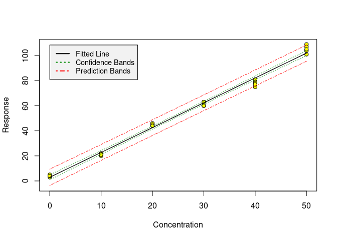
If you use unweighted regression, as in the above example, we can calculate a Limit Of Detection (LOD) from the calibration data.
lod(m0)
#> $x
#> [1] 5.407085
#>
#> $y
#> [1] 13.63911
This is the minimum detectable value (German: Erfassungsgrenze), i.e. the value where the probability that the signal is not detected although the analyte is present is below a specified error tolerance beta (default is 0.05 following the IUPAC recommendation).
You can also calculate the decision limit (German: Nachweisgrenze), i.e. the value that is significantly different from the blank signal with an error tolerance alpha (default is 0.05, again following IUPAC recommendations) by setting beta to 0.5.
lod(m0, beta = 0.5)
#> $x
#> [1] 2.720388
#>
#> $y
#> [1] 8.314841
Furthermore, you can calculate the Limit Of Quantification (LOQ), being defined as the value where the relative error of the quantification given the calibration model reaches a prespecified value (default is 1/3).
loq(m0)
#> $x
#> [1] 9.627349
#>
#> $y
#> [1] 22.00246Finally, you can get a confidence interval for the values measured
using the calibration curve, i.e. for the inverse predictions using the
function inverse.predict.
inverse.predict(m0, 90)
#> $Prediction
#> [1] 43.93983
#>
#> $`Standard Error`
#> [1] 1.576985
#>
#> $Confidence
#> [1] 3.230307
#>
#> $`Confidence Limits`
#> [1] 40.70952 47.17014
If you have replicate measurements of the same sample, you can also give a vector of numbers.
inverse.predict(m0, c(91, 89, 87, 93, 90))
#> $Prediction
#> [1] 43.93983
#>
#> $`Standard Error`
#> [1] 0.796884
#>
#> $Confidence
#> [1] 1.632343
#>
#> $`Confidence Limits`
#> [1] 42.30749 45.57217You can use the R help system to view documentation, or you can have a look at the online documentation.