![]()
This package implements A-Spline regression, an adaptive procedure for fitting splines with automatic selection of the knots. One-dimentional B-Splines of any non-negative degree can be fitted. This method uses a penalization approach to compensate overfitting. The penalty is proportional to the number of knots used to support the regression spline. Consequently, the fitted splines will have knots only where necessary and the fitted model is sparser than comparable penalized spline regressions (for instance the standard method for penalized splines: P-splines).
You can install the development version from GitHub with:
# install.packages("devtools")
devtools::install_github("goepp/aspline")Below is an illustration of the A-spline procedure using the helmet data. The thick line represents the fitted spline and the thin line represents the B-spline basis decomposition of the fitted curve.
library(aspline)
library(tidyverse)
#> ── Attaching packages ─────────────────────────────────────── tidyverse 1.3.1 ──
#> ✓ ggplot2 3.3.3     ✓ purrr   0.3.4
#> ✓ tibble  3.1.2     ✓ dplyr   1.0.5
#> ✓ tidyr   1.1.3     ✓ stringr 1.4.0
#> ✓ readr   1.4.0     ✓ forcats 0.5.1
#> ── Conflicts ────────────────────────────────────────── tidyverse_conflicts() ──
#> x dplyr::filter() masks stats::filter()
#> x dplyr::lag()    masks stats::lag()
library(splines2)
data(helmet)
x <- helmet$x
y <- helmet$y
k <- 40
knots <- seq(min(x), max(x), length = k + 2)[-c(1, k + 2)]
degree <- 3
pen <- 10 ^ seq(-4, 4, 0.25)
x_seq <- seq(min(x), max(x), length = 1000)
aridge <- aspline(x, y, knots, pen, degree = degree)
#> Warning: `data_frame()` was deprecated in tibble 1.1.0.
#> Please use `tibble()` instead.
a_fit <- lm(y ~ bSpline(x, knots = aridge$knots_sel[[which.min(aridge$ebic)]],
                        degree = degree))
X_seq <- bSpline(x_seq, knots = aridge$knots_sel[[which.min(aridge$ebic)]],
                 intercept = TRUE, degree = degree)
a_basis <- (X_seq %*% diag(coef(a_fit))) %>%
  as.data.frame() %>%
  mutate(x = x_seq) %>%
  reshape2::melt(id.vars = "x", variable.name = "spline_n", value.name = "y") %>%
  as_tibble() %>%
  filter(y != 0)
a_predict <- data_frame(x = x_seq, pred = predict(a_fit, data.frame(x = x_seq)))
ggplot() +
  geom_point(data = helmet, aes(x, y), shape = 1) +
  geom_line(data = a_predict, aes(x, pred), size = 0.5) +
  geom_line(data = a_basis, aes(x, y, group = spline_n), linetype = 1, size = 0.1) +
  theme(legend.position = "none") +
  ylab("") +
  xlab("")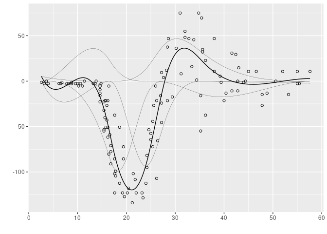
For the sake of comparision, we display here the estimated P-spline with the same data. The thin lines also represent the B-spline basis decomposition.
p_fit <- mgcv::gam(y ~ s(x, bs = "ps", k = length(knots) + 3 + 1, m = c(3, 2)))
X <- bSpline(x_seq, knots = knots, intercept = TRUE)
p_basis <- (X %*% diag(coef(p_fit))) %>%
  as.data.frame() %>%
  mutate(x = x_seq) %>%
  reshape2::melt(id.vars = "x", variable.name = "spline_n", value.name = "y") %>%
  as_tibble() %>%
  filter(y != 0)
p_predict <- data_frame(x = x_seq, pred = predict(p_fit, data.frame(x = x_seq)))
ggplot() +
  geom_point(data = helmet, aes(x, y), shape = 1) +
  geom_line(data = p_predict, aes(x, pred), size = 0.5) +
  geom_line(data = p_basis, aes(x, y, group = spline_n), linetype = 1, size = 0.1) +
  theme(legend.position = "none") +
  ylab("") + xlab("")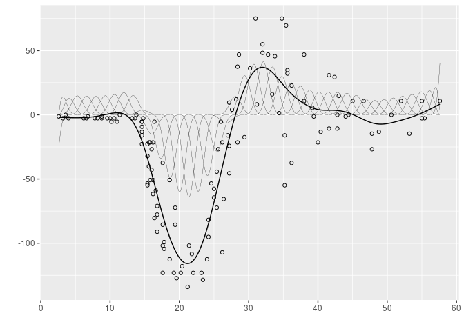
If you encounter a bug or have a suggestion for improvement, please raise an issue or make a pull request.
This package is released under the GPLv3 License: see the
LICENSE file or the online text. In
short,
you can use, modify, and distribute (including for commerical use) this
package, with the notable obligations to use the GPLv3 license for your
work and to provide a copy of the present source code.