
![]()
![]()


![]()
Fit, interpret, and make predictions with oblique random forests (RFs).
Fast and versatile tools for oblique RFs.1
Accurate predictions.2
Intuitive design with formula based interface.
Extensive input checks and informative error messages.
Compatible with tidymodels and
mlr3
You can install aorsf from CRAN using
install.packages("aorsf")You can install the development version of aorsf from GitHub with:
# install.packages("remotes")
remotes::install_github("ropensci/aorsf")library(aorsf)
library(tidyverse)aorsf fits several types of oblique RFs with the
orsf() function, including classification, regression, and
survival RFs.
For classification, we fit an oblique RF to predict penguin species
using penguin data from the magnificent
palmerpenguins R package
# An oblique classification RF
penguin_fit <- orsf(data = penguins_orsf,
                    n_tree = 5,
                    formula = species ~ .)

penguin_fit
#> ---------- Oblique random classification forest
#>
#>      Linear combinations: Accelerated Logistic regression
#>           N observations: 333
#>                N classes: 3
#>                  N trees: 5
#>       N predictors total: 7
#>    N predictors per node: 3
#>  Average leaves per tree: 6
#> Min observations in leaf: 5
#>           OOB stat value: 0.99
#>            OOB stat type: AUC-ROC
#>      Variable importance: anova
#>
#> -----------------------------------------
For regression, we use the same data but predict bill length of penguins:
# An oblique regression RF
bill_fit <- orsf(data = penguins_orsf,
                 n_tree = 5,
                 formula = bill_length_mm ~ .)

bill_fit
#> ---------- Oblique random regression forest
#>
#>      Linear combinations: Accelerated Linear regression
#>           N observations: 333
#>                  N trees: 5
#>       N predictors total: 7
#>    N predictors per node: 3
#>  Average leaves per tree: 42.6
#> Min observations in leaf: 5
#>           OOB stat value: 0.76
#>            OOB stat type: RSQ
#>      Variable importance: anova
#>
#> -----------------------------------------
My personal favorite is the oblique survival RF with accelerated Cox
regression because it was the first type of oblique RF that
aorsf provided (see JCGS paper).
Here, we use it to predict mortality risk following diagnosis of primary
biliary cirrhosis:
# An oblique survival RF
pbc_fit <- orsf(data = pbc_orsf,
                n_tree = 5,
                formula = Surv(time, status) ~ . - id)

pbc_fit
#> ---------- Oblique random survival forest
#>
#>      Linear combinations: Accelerated Cox regression
#>           N observations: 276
#>                 N events: 111
#>                  N trees: 5
#>       N predictors total: 17
#>    N predictors per node: 5
#>  Average leaves per tree: 20.4
#> Min observations in leaf: 5
#>       Min events in leaf: 1
#>           OOB stat value: 0.79
#>            OOB stat type: Harrell's C-index
#>      Variable importance: anova
#>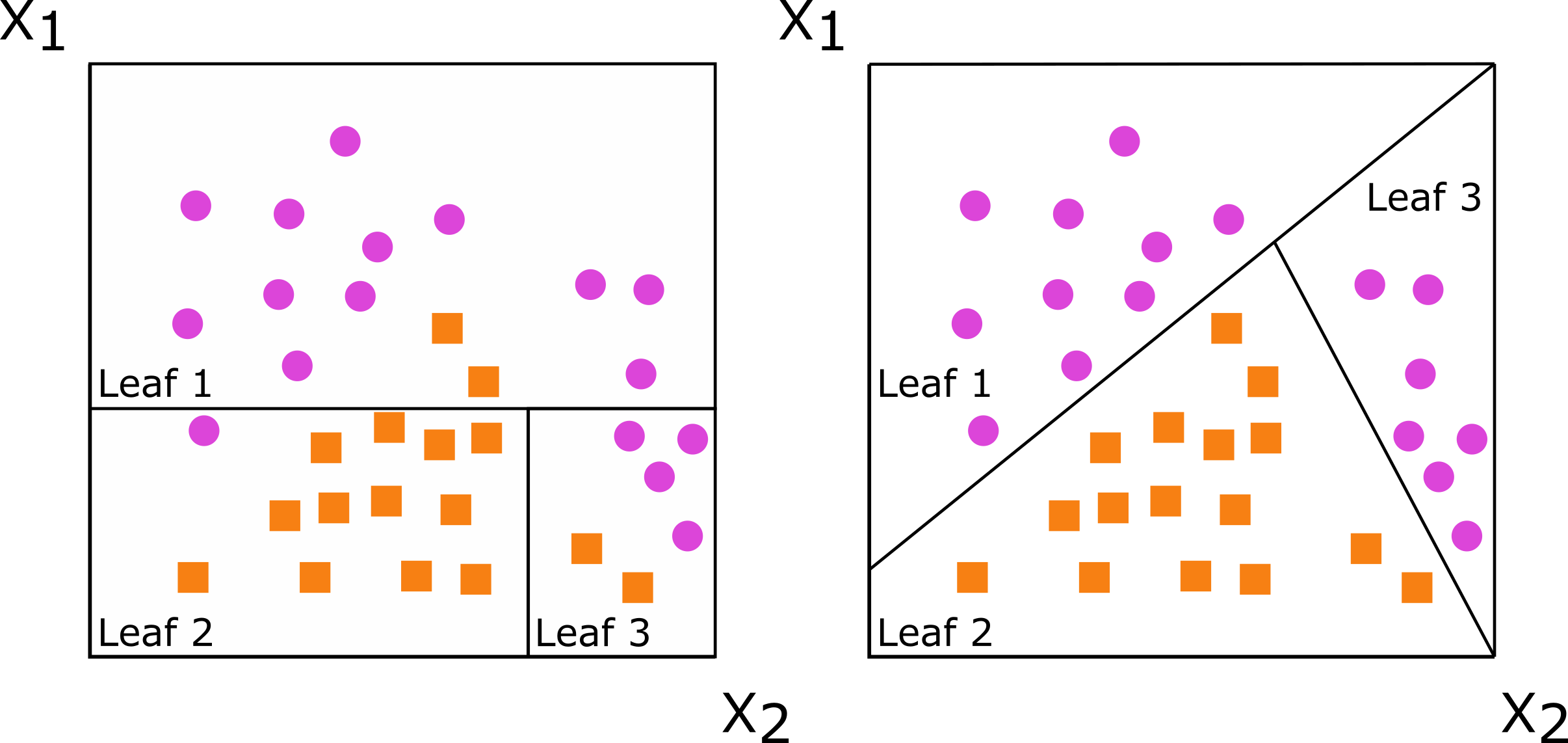
#> -----------------------------------------Decision trees are grown by splitting a set of training data into non-overlapping subsets, with the goal of having more similarity within the new subsets than between them. When subsets are created with a single predictor, the decision tree is axis-based because the subset boundaries are perpendicular to the axis of the predictor. When linear combinations (i.e., a weighted sum) of variables are used instead of a single variable, the tree is oblique because the boundaries are neither parallel nor perpendicular to the axis.
Figure: Decision trees for classification with axis-based splitting (left) and oblique splitting (right). Cases are orange squares; controls are purple circles. Both trees partition the predictor space defined by variables X1 and X2, but the oblique splits do a better job of separating the two classes.
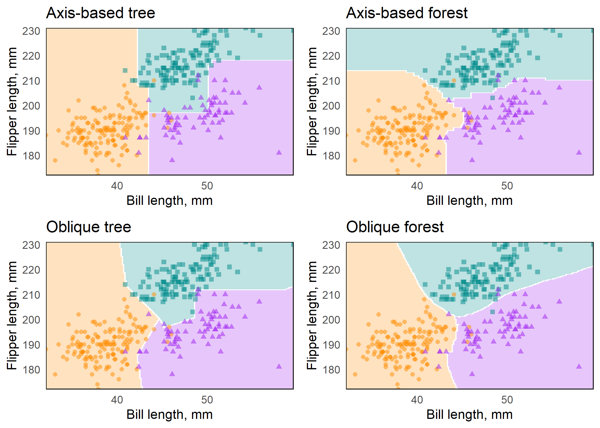
So, how does this difference translate to real data, and how does it
impact random forests comprising hundreds of axis-based or oblique
trees? We will demonstrate this using the penguin
data.3 We will also use this function to make several
plots:
plot_decision_surface <- function(predictions, title, grid){

 # this is not a general function for plotting
 # decision surfaces. It just helps to minimize
 # copying and pasting of code.

 class_preds <- bind_cols(grid, predictions) %>%
  pivot_longer(cols = c(Adelie,
                        Chinstrap,
                        Gentoo)) %>%
  group_by(flipper_length_mm, bill_length_mm) %>%
  arrange(desc(value)) %>%
  slice(1)

 cols <- c("darkorange", "purple", "cyan4")

 ggplot(class_preds, aes(bill_length_mm, flipper_length_mm)) +
  geom_contour_filled(aes(z = value, fill = name),
                      alpha = .25) +
  geom_point(data = penguins_orsf,
             aes(color = species, shape = species),
             alpha = 0.5) +
  scale_color_manual(values = cols) +
  scale_fill_manual(values = cols) +
  labs(x = "Bill length, mm",
       y = "Flipper length, mm") +
  theme_minimal() +
  scale_x_continuous(expand = c(0,0)) +
  scale_y_continuous(expand = c(0,0)) +
  theme(panel.grid = element_blank(),
        panel.border = element_rect(fill = NA),
        legend.position = '') +
  labs(title = title)

}
We also use a grid of points for plotting decision surfaces:
grid <- expand_grid(

 flipper_length_mm = seq(min(penguins_orsf$flipper_length_mm),
                     max(penguins_orsf$flipper_length_mm),
                  len = 200),
 bill_length_mm = seq(min(penguins_orsf$bill_length_mm),
                      max(penguins_orsf$bill_length_mm),
                      len = 200)
)
We use orsf with mtry=1 to fit axis-based
trees:
fit_axis_tree <- penguins_orsf %>%
 orsf(species ~ bill_length_mm + flipper_length_mm,
      n_tree = 1,
      mtry = 1,
      tree_seeds = 106760)
Next we use orsf_update to copy and modify the original
model, expanding it to fit an oblique tree by using mtry=2
instead of mtry=1, and to include 500 trees instead of
1:
fit_axis_forest <- fit_axis_tree %>%
 orsf_update(n_tree = 500)

fit_oblique_tree <- fit_axis_tree %>%
 orsf_update(mtry = 2)

fit_oblique_forest <- fit_oblique_tree %>%
 orsf_update(n_tree = 500)
And now we have all we need to visualize decision surfaces using predictions from these four fits:
preds <- list(fit_axis_tree,
              fit_axis_forest,
              fit_oblique_tree,
              fit_oblique_forest) %>%
 map(predict, new_data = grid, pred_type = 'prob')

titles <- c("Axis-based tree",
            "Axis-based forest",
            "Oblique tree",
            "Oblique forest")

plots <- map2(preds, titles, plot_decision_surface, grid = grid)Figure: Axis-based and oblique decision surfaces from a single tree and an ensemble of 500 trees. Axis-based trees have boundaries perpendicular to predictor axes, whereas oblique trees can have boundaries that are neither parallel nor perpendicular to predictor axes. Axis-based forests tend to have ‘step-function’ decision boundaries, while oblique forests tend to have smooth decision boundaries.
The importance of individual predictor variables can be estimated in
three ways using aorsf and can be used on any type of
oblique RF. Also, variable importance functions always return a named
character vector
negation2: Each variable is assessed separately by multiplying the variable’s coefficients by -1 and then determining how much the model’s performance changes. The worse the model’s performance after negating coefficients for a given variable, the more important the variable. This technique is promising b/c it does not require permutation and it emphasizes variables with larger coefficients in linear combinations, but it is also relatively new and hasn’t been studied as much as permutation importance. See Jaeger, (2023) for more details on this technique.
orsf_vi_negate(pbc_fit)
#>          bili        copper         stage           sex           age
#>  0.1552460736  0.1156218837  0.0796917628  0.0533427094  0.0283132385
#>       albumin           trt          chol      alk.phos      platelet
#>  0.0279823814  0.0168238416  0.0153010749  0.0148718669  0.0094582765
#>         edema       ascites       spiders       protime        hepato
#>  0.0067975986  0.0065505801  0.0062356214 -0.0004653046 -0.0026664147
#>           ast          trig
#> -0.0028902524 -0.0106616501permutation: Each variable is assessed separately by randomly permuting the variable’s values and then determining how much the model’s performance changes. The worse the model’s performance after permuting the values of a given variable, the more important the variable. This technique is flexible, intuitive, and frequently used. It also has several known limitations
orsf_vi_permute(penguin_fit)
#>    bill_length_mm     bill_depth_mm       body_mass_g            island
#>       0.121351910       0.101846889       0.097822451       0.080772909
#>               sex flipper_length_mm              year
#>       0.035053517       0.008270751      -0.008058339
analysis of variance (ANOVA)4: A p-value is computed for each coefficient in each linear combination of variables in each decision tree. Importance for an individual predictor variable is the proportion of times a p-value for its coefficient is < 0.01. This technique is very efficient computationally, but may not be as effective as permutation or negation in terms of selecting signal over noise variables. See Menze, 2011 for more details on this technique.
orsf_vi_anova(bill_fit)
#>           species               sex     bill_depth_mm flipper_length_mm
#>        0.51652893        0.27906977        0.06315789        0.04950495
#>       body_mass_g            island              year
#>        0.04807692        0.02687148        0.00000000
You can supply your own R function to estimate out-of-bag error (see oob vignette) or to estimate out-of-bag variable importance (see orsf_vi examples)
Partial dependence (PD) shows the expected prediction from a model as
a function of a single predictor or multiple predictors. The expectation
is marginalized over the values of all other predictors, giving
something like a multivariable adjusted estimate of the model’s
prediction.. You can use specific values for a predictor to compute PD
or let aorsf pick reasonable values for you if you use
pred_spec_auto():
# pick your own values
orsf_pd_oob(bill_fit, pred_spec = list(species = c("Adelie", "Gentoo")))
#>    species     mean      lwr     medn      upr
#>     <fctr>    <num>    <num>    <num>    <num>
#> 1:  Adelie 39.99394 35.76532 39.80782 46.13931
#> 2:  Gentoo 46.66565 40.02938 46.88517 51.61367

# let aorsf pick reasonable values for you:
orsf_pd_oob(bill_fit, pred_spec = pred_spec_auto(bill_depth_mm, island))
#>     bill_depth_mm    island     mean      lwr     medn      upr
#>             <num>    <fctr>    <num>    <num>    <num>    <num>
#>  1:          14.3    Biscoe 43.94960 35.90421 45.30159 51.05109
#>  2:          15.6    Biscoe 44.24705 36.62759 45.57321 51.08020
#>  3:          17.3    Biscoe 44.84757 36.53804 45.62910 53.93833
#>  4:          18.7    Biscoe 45.08939 36.35893 46.16893 54.42075
#>  5:          19.5    Biscoe 45.13608 36.21033 46.08023 54.42075
#> ---
#> 11:          14.3 Torgersen 43.55984 35.47143 44.18127 51.05109
#> 12:          15.6 Torgersen 43.77317 35.44683 44.28406 51.08020
#> 13:          17.3 Torgersen 44.56465 35.84585 44.83694 53.93833
#> 14:          18.7 Torgersen 44.68367 35.44010 44.86667 54.42075
#> 15:          19.5 Torgersen 44.64605 35.44010 44.86667 54.42075
The summary function, orsf_summarize_uni(), computes PD
for as many variables as you ask it to, using sensible values.
orsf_summarize_uni(pbc_fit, n_variables = 2)
#>
#> -- bili (VI Rank: 1) -----------------------------
#>
#>         |----------------- Risk -----------------|
#>   Value      Mean     Median     25th %    75th %
#>  <char>     <num>      <num>      <num>     <num>
#>    0.60 0.2098108 0.07168855 0.01138461 0.2860450
#>    0.80 0.2117933 0.07692308 0.01709469 0.2884990
#>    1.40 0.2326560 0.08445419 0.02100837 0.3563622
#>    3.55 0.4265979 0.35820106 0.05128824 0.7342923
#>    7.30 0.4724608 0.44746241 0.11759259 0.8039683
#>
#> -- copper (VI Rank: 2) ---------------------------
#>
#>         |----------------- Risk -----------------|
#>   Value      Mean     Median     25th %    75th %
#>  <char>     <num>      <num>      <num>     <num>
#>    25.0 0.2332412 0.04425936 0.01587919 0.3888304
#>    42.5 0.2535448 0.07417582 0.01754386 0.4151786
#>    74.0 0.2825471 0.11111111 0.01988069 0.4770833
#>     130 0.3259604 0.18771003 0.04658385 0.5054348
#>     217 0.4213303 0.28571429 0.13345865 0.6859423
#>
#>  Predicted risk at time t = 1788 for top 2 predictors
For more on PD, see the vignette
Unlike partial dependence, which shows the expected prediction as a function of one or multiple predictors, individual conditional expectations (ICE) show the prediction for an individual observation as a function of a predictor.
For more on ICE, see the vignette
The orsf_vint() function computes a score for each
possible interaction in a model based on PD using the method described
in Greenwell et al, 2018.5 It can be slow for larger
datasets, but substantial speedups occur by making use of
multi-threading and restricting the search to a smaller set of
predictors.
preds_interaction <- c("albumin", "protime", "bili", "spiders", "trt")

# While it is tempting to speed up `orsf_vint()` by growing a smaller
# number of trees, results may become unstable with this shortcut.
pbc_interactions <- pbc_fit %>%
 orsf_update(n_tree = 500, tree_seeds = 329) %>%
 orsf_vint(n_thread = 0,  predictors = preds_interaction)

pbc_interactions
#>          interaction      score
#>               <char>      <num>
#>  1: albumin..protime 0.97837184
#>  2:    protime..bili 0.78999788
#>  3:    albumin..bili 0.59128756
#>  4:    bili..spiders 0.13192184
#>  5:        bili..trt 0.13192184
#>  6: albumin..spiders 0.06578222
#>  7:     albumin..trt 0.06578222
#>  8: protime..spiders 0.03012718
#>  9:     protime..trt 0.03012718
#> 10:     spiders..trt 0.00000000
What do the values in score mean? These values are the
average of the standard deviation of the standard deviation of PD in one
variable conditional on the other variable. They should be interpreted
relative to one another, i.e., a higher scoring interaction is more
likely to reflect a real interaction between two variables than a lower
scoring one.
Do these interaction scores make sense? Let’s test the top scoring
and lowest scoring interactions using coxph().
library(survival)
# the top scoring interaction should get a lower p-value
anova(coxph(Surv(time, status) ~ protime * albumin, data = pbc_orsf))
#> Analysis of Deviance Table
#>  Cox model: response is Surv(time, status)
#> Terms added sequentially (first to last)
#>
#>                  loglik  Chisq Df Pr(>|Chi|)
#> NULL            -550.19
#> protime         -538.51 23.353  1  1.349e-06 ***
#> albumin         -514.89 47.255  1  6.234e-12 ***
#> protime:albumin -511.76  6.252  1    0.01241 *
#> ---
#> Signif. codes:  0 '***' 0.001 '**' 0.01 '*' 0.05 '.' 0.1 ' ' 1
# the bottom scoring interaction should get a higher p-value
anova(coxph(Surv(time, status) ~ spiders * trt, data = pbc_orsf))
#> Analysis of Deviance Table
#>  Cox model: response is Surv(time, status)
#> Terms added sequentially (first to last)
#>
#>              loglik   Chisq Df Pr(>|Chi|)
#> NULL        -550.19
#> spiders     -538.58 23.2159  1  1.448e-06 ***
#> trt         -538.39  0.3877  1     0.5335
#> spiders:trt -538.29  0.2066  1     0.6494
#> ---
#> Signif. codes:  0 '***' 0.001 '**' 0.01 '*' 0.05 '.' 0.1 ' ' 1
Note: this is exploratory and not a true null hypothesis test. Why?
Because we used the same data both to generate and to test the null
hypothesis. We are not so much conducting statistical inference when we
test these interactions with coxph as we are demonstrating
the interaction scores that orsf_vint() provides are
consistent with tests from other models.
For survival analysis, comparisons between aorsf and
existing software are presented in our JCGS paper. The
paper:
describes aorsf in detail with a summary of the
procedures used in the tree fitting algorithm
runs a general benchmark comparing aorsf with
obliqueRSF and several other learners
reports prediction accuracy and computational efficiency of all learners.
runs a simulation study comparing variable importance techniques with oblique survival RFs, axis based survival RFs, and boosted trees.
reports the probability that each variable importance technique will rank a relevant variable with higher importance than an irrelevant variable.
The developers of aorsf received financial support from
the Center for Biomedical Informatics, Wake Forest University School of
Medicine. We also received support from the National Center for
Advancing Translational Sciences of the National Institutes of Health
under Award Number UL1TR001420.
The content is solely the responsibility of the authors and does not necessarily represent the official views of the National Institutes of Health.