![]()
![]()
SDMtune provides a user-friendly framework that enables the training and the evaluation of species distribution models (SDMs). The package implements functions for data driven variable selection and model tuning and includes numerous utilities to display the results. All the functions used to select variables or to tune model hyperparameters have an interactive real-time chart displayed in the RStudio viewer pane during their execution. Visit the package website and learn how to use SDMtune starting from the first article Prepare data for the analysis.
You can install the latest release version from CRAN:
install.packages("SDMtune")Or the development version from GitHub:
devtools::install_github("ConsBiol-unibern/SDMtune")SDMtune implements three functions for hyperparameters tuning:
gridSearch: runs all the possible combinations of
predefined hyperparameters’ values;randomSearch: randomly selects a fraction of the
possible combinations of predefined hyperparameters’ values;optimizeModel: uses a genetic algorithm that
aims to optimize the given evaluation metric by combining the predefined
hyperparameters’ values.When the amount of hyperparameters’ combinations is high, the
computation time necessary to train all the defined models could be very
long. The function optimizeModel offers a valid alternative
that reduces computation time thanks to an implemented genetic
algorithm. This function seeks the best combination of
hyperparameters reaching a near optimal or optimal solution in a reduced
amount of time compared to gridSearch. The following code
shows an example using a simulated dataset. First a model is trained
using the Maxnet algorithm implemented in the
maxnet package with default hyperparameters’ values. After
the model is trained, both the gridSearch and
optimizeModel functions are executed to compare the
execution time and model performance evaluated with the AUC metric. If
the following code is not clear, please check the articles in the website.
library(SDMtune)

# Acquire environmental variables
files <- list.files(path = file.path(system.file(package = "dismo"), "ex"),
                    pattern = "grd", full.names = TRUE)
predictors <- terra::rast(files)

# Prepare presence and background locations
p_coords <- virtualSp$presence
bg_coords <- virtualSp$background

# Create SWD object
data <- prepareSWD(species = "Virtual species", p = p_coords, a = bg_coords,
                   env = predictors, categorical = "biome")

# Split presence locations in training (80%) and testing (20%) datasets
datasets <- trainValTest(data, test = 0.2, only_presence = TRUE, seed = 25)
train <- datasets[[1]]
test <- datasets[[2]]

# Train a Maxnet model
model <- train(method = "Maxnet", data = train)

# Define the hyperparameters to test
h <- list(reg = seq(0.1, 3, 0.1), fc = c("lq", "lh", "lqp", "lqph", "lqpht"))

# Test all the possible combinations with gridSearch
gs <- gridSearch(model, hypers = h, metric = "auc", test = test)
head(gs@results[order(-gs@results$test_AUC), ])  # Best combinations

# Use the genetic algorithm instead with optimizeModel
om <- optimizeModel(model, hypers = h, metric = "auc", test = test, seed = 4)
head(om@results)  # Best combinations
During the execution of “tuning” and “variable selection” functions,
real-time charts displaying training and validation metrics are
displayed in the RStudio viewer pane (below is a screencast of the
previous executed optimizeModel function).
In the following example we train a Maxent model:
# Train a Maxent model
sdmtune_model <- train(method = "Maxent", data = data)
We compare the execution time of the predict function
between SDMtune that uses its own algorithm and
dismo (Hijmans et al. 2017) that calls the MaxEnt Java
software (Phillips, Anderson, and Schapire 2006). We first convert the
object sdmtune_model in a object that is accepted by
dismo:
maxent_model <- SDMmodel2MaxEnt(sdmtune_model)Next is a function used below to test if the results are equal, with
a tolerance of 1e-7:
my_check <- function(values) {
  return(all.equal(values[[1]], values[[2]], tolerance = 1e-7))
}
Now we test the execution time using the microbenckmark package:
bench <- microbenchmark::microbenchmark(
  SDMtune = predict(sdmtune_model, data = data, type = "cloglog"),
  dismo = predict(maxent_model, data@data),
  check = my_check
)
and plot the output:
library(ggplot2)
ggplot(bench, aes(x = expr, y = time/1000000, fill = expr)) +
  geom_boxplot() +
  labs(fill = "", x = "Package", y = "time (milliseconds)") +
  theme_minimal()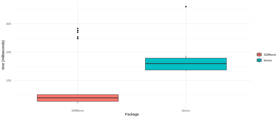
To train a Maxent model using the Java implementation you need that:
You can check the version of MaxEnt used by dismo with
the following command:
dismo::maxent()The MaxEnt jar file used by dismo is
located in the folder returned by the following command:
system.file(package="dismo")In case you want to upgrade to a newer version of MaxEnt (if available), download the file maxent.jar here and replace the file already present in the previous folder.
The function checkMaxentInstallation checks that Java
JDK and rJava are installed, and that the file maxent.jar is in the
correct folder.
checkMaxentInstallation()If everything is correctly configured for dismo, the
command dismo::maxent() will return the new MaxEnt
version.
Please note that this project follows a Contributor Code of Conduct. By contributing to this project, you agree to abide by its terms.