| Project | Main branch | Devel branch |
|---|---|---|
 |
||
Functions for calculating life history metrics from matrix population models (MPMs).
Includes functions for:
Install the stable release package from CRAN with:
install.packages("Rage")Install from GitHub with:
# install.packages("remotes")
remotes::install_github("jonesor/Rage")library(Rage)The functions in Rage work on MPMs (or components of MPMs), so we’ll
start by loading one of the example MPMs included in the Rage package
(mpm1).
library(Rage) # load Rage
data(mpm1) # load data object 'mpm1'

mpm1
#> $matU
#>         seed small medium large dormant
#> seed    0.10  0.00   0.00  0.00    0.00
#> small   0.05  0.12   0.10  0.00    0.00
#> medium  0.00  0.35   0.12  0.23    0.12
#> large   0.00  0.03   0.28  0.52    0.10
#> dormant 0.00  0.00   0.16  0.11    0.17
#>
#> $matF
#>         seed small medium large dormant
#> seed       0     0   17.9  45.6       0
#> small      0     0    0.0   0.0       0
#> medium     0     0    0.0   0.0       0
#> large      0     0    0.0   0.0       0
#> dormant    0     0    0.0   0.0       0
The object mpm1 is a list containing two elements: the
growth/survival component of the MPM (the U matrix),
and the sexual reproduction component (the F matrix).
We can obtain the full MPM by adding the two components together
(A = U + F).
One of the most common arguments among functions in Rage is
start, which is used to specify the stage class that
represents the ‘beginning of life’ for the purposes of calculation.
Because the first stage class in mpm1 is a ‘seed’ stage,
which we might consider functionally-distinct from the ‘above-ground’
stages, we’ll specify start = 2 to set our starting stage
class of interest to the ‘small’ stage.
life_expect_mean(mpm1$matU, start = 2) # life expectancy
#> [1] 2.509116
longevity(mpm1$matU, start = 2, lx_crit = 0.05) # longevity (age at lx = 0.05)
#> [1] 7
mature_age(mpm1$matU, mpm1$matF, start = 2) # mean age at first reproduction
#>    small
#> 2.136364
mature_prob(mpm1$matU, mpm1$matF, start = 2) # prob survival to first repro
#> [1] 0.4318182
Some life history traits are independent of the starting stage class,
in which case we don’t need to specify start.
net_repro_rate(mpm1$matU, mpm1$matF) # net reproductive rate
#> [1] 1.852091
gen_time(mpm1$matU, mpm1$matF) # generation time
#> [1] 5.394253
Some life history traits are calculated from a life table rather than
an MPM. For example, traits like entropy (entropy_k_stage)
and shape measures (shape_surv, shape_rep)
etc. In these cases, the calculation of age trajectories (lx and or mx
trajectories) is handled internally. Nevertheless, it can still be
useful to obtain the trajectories directly, in which case we can first
use the mpm_to_ group of functions.
# first derive age-trajectories of survivorship (lx) and fecundity (mx)
lx <- mpm_to_lx(mpm1$matU, start = 2)
mx <- mpm_to_mx(mpm1$matU, mpm1$matF, start = 2)Some MPMs are parameterized with a stasis loop at the maximum stage
class, which can lead to apparent plateaus in mortality or fertility
trajectories derived using age-from-stage methods. The function
qsd_converge() can be used to identify the time it takes
for a cohort to reach the quasi-stationary distribution (QSD). This
quantity can then be used to subset age trajectories of mortality or
fertility to periods earlier than the QSD, so as to avoid artefactual
plateaus in mortality or fertility.
# derive life table from MPM
lt <- mpm_to_table(mpm1$matU, start = 2)

# calculate time to QSD
(q <- qsd_converge(mpm1$matU, start = 2))
#> [1] 6

# plot mortality trajectory w/ vertical line at time to QSD
par(mar = c(4.5, 4.5, 1, 1))
plot(qx ~ x, data = lt, type = "l", ylim = c(0, 0.65))
abline(v = q, lty = 2)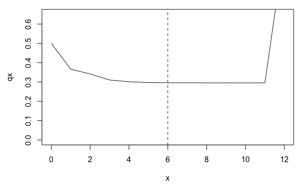
From the life table derived from mpm1, we can see a
plateau in the mortality rate (qx) beginning around age 5. However, this
plateau corresponds to the QSD and is therefore probably an artefact of
the stasis loop rather than a biological reality for the population
represented by mpm1.
One approach to accounting for this artefactual plateau in subsequent life history calculations is to limit our life table to the period prior to the QSD.
# calculate the shape of the survival/mortality trajectory
shape_surv(lt$lx) # based on full lx trajectory
#> [1] -0.04681254
shape_surv(lt$lx[1:q]) # based on lx trajectory prior to the QSD
#> [1] -0.06573764The transition rates that make up MPMs generally reflect products of two or more vital rates (sometimes called ‘lower-level vital rates’). Assuming a post-breeding census design, we can retroactively break apart each transition rate into at least two vital rate components: survival, and ‘something’ conditional on survival. That ‘something’ might be growth, shrinkage, stasis, dormancy, fecundity, or clonality.
To summarize vital rates within stage classes, we can use
the vr_vec_ group of functions. We’ll use the
exclude argument here to exclude certain stage classes
(‘seed’ and ‘dormant’) from the calculation of certain vital rates
(e.g. we don’t consider the large-to-dormant transition to actually
represent ‘growth’).
vr_vec_survival(mpm1$matU)
#>    seed   small  medium   large dormant
#>    0.15    0.50    0.66    0.86    0.39
vr_vec_growth(mpm1$matU, exclude = c(1, 5))
#>      seed     small    medium     large   dormant
#>        NA 0.7600000 0.4242424        NA        NA
vr_vec_shrinkage(mpm1$matU, exclude = 5)
#>      seed     small    medium     large   dormant
#>        NA        NA 0.1515152 0.2674419        NA
vr_vec_stasis(mpm1$matU)
#>      seed     small    medium     large   dormant
#> 0.6666667 0.2400000 0.1818182 0.6046512 0.4358974
vr_vec_dorm_enter(mpm1$matU, dorm_stages = 5)
#>      seed     small    medium     large   dormant
#>        NA        NA 0.2424242 0.1279070        NA
vr_vec_dorm_exit(mpm1$matU, dorm_stages = 5)
#>      seed     small    medium     large   dormant
#>        NA        NA        NA        NA 0.5641026
vr_vec_reproduction(mpm1$matU, mpm1$matF)
#>     seed    small   medium    large  dormant
#> NA NA 27.12121 53.02326 NATo summarize vital rates across stage classes, we can use
the vr_ group of functions. By default these functions take
a simple average of the stage-specific vital rates produced by the
corresponding vr_vec_ function. However, here we’ll
demonstrate how to specify a weighted average across stages,
based on the stable stage distribution at equilibrium (w).
# derive full MPM (matA)
mpm1$matA <- mpm1$matU + mpm1$matF

# calculate stable stage distribution at equilibrium using popdemo::eigs
library(popdemo)
#> Welcome to popdemo! This is version 1.3-0
#> Use ?popdemo for an intro, or browseVignettes('popdemo') for vignettes
#> Citation for popdemo is here: doi.org/10.1111/j.2041-210X.2012.00222.x
#> Development and legacy versions are here: github.com/iainmstott/popdemo
w <- popdemo::eigs(mpm1$matA, what = "ss")

# calculate MPM-specific vital rates
vr_survival(mpm1$matU, exclude_col = c(1, 5), weights_col = w)
#> [1] 0.5963649
vr_growth(mpm1$matU, exclude = c(1, 5), weights_col = w)
#> [1] 0.6602975
vr_shrinkage(mpm1$matU, exclude = c(1, 5), weights_col = w)
#> [1] 0.1960601
vr_stasis(mpm1$matU, exclude = c(1, 5), weights_col = w)
#> [1] 0.2824323
vr_dorm_enter(mpm1$matU, dorm_stages = 5, weights_col = w)
#> [1] 0.1984209
vr_dorm_exit(mpm1$matU, dorm_stages = 5, weights_col = w)
#> [1] 0.5641026
vr_fecundity(mpm1$matU, mpm1$matF, weights_col = w)
#> [1] 37.07409
Note how we’ve chosen to exclude the ‘seed’ and ‘dormant’ stage classes from our vital rate summaries, because we consider these to be special classes (e.g. ‘growth’ from the ‘seed’ stage is really ‘germination’, which we may think of as separate from somatic growth from ‘small’ to ‘medium’, or ‘medium’ to ‘large’).
The perturb_matrix() function measures the response of a
demographic statistic to perturbation of individual matrix elements
(i.e. sensitivities and elasticities). The perturb_vr() and
perturb_trans() functions implement perturbation analyses
by vital rate type (survival, growth, etc.) and transition type (stasis,
retrogression, etc.), respectively.
# matrix element perturbation
perturb_matrix(mpm1$matA, type = "sensitivity")
#>               seed      small      medium       large     dormant
#> seed     0.2173031 0.01133203 0.004786308 0.002986833 0.001150703
#> small    4.4374613 0.23140857 0.097739870 0.060993320 0.023498191
#> medium  10.8654599 0.56661979 0.239323184 0.149346516 0.057537001
#> large   21.3053309 1.11104269 0.469270739 0.292842885 0.112820081
#> dormant  3.6111989 0.18831947 0.079540419 0.049636195 0.019122779

# vital rate perturbation
# (we use as.data.frame here for prettier printing)
as.data.frame(perturb_vr(mpm1$matU, mpm1$matF, type = "sensitivity"))
#>   survival   growth  shrinkage  fecundity clonality
#> 1 2.986054 1.077597 -0.1653284 0.00572764         0

# transition type perturbation
as.data.frame(perturb_trans(mpm1$matU, mpm1$matF, type = "sensitivity"))
#>     stasis     retro    progr   fecundity clonality
#> 1 1.000001 0.4174435 6.713571 0.007773141 NARage includes a variety of functions that can be used to manipulate
or transform MPMs. For example, we can collapse an MPM to a smaller
number of stage classes using mpm_collapse().
# collapse 'small', 'medium', and 'large' stages into single stage class
col1 <- mpm_collapse(mpm1$matU, mpm1$matF, collapse = list(1, 2:4, 5))
col1$matA
#>      [,1]        [,2] [,3]
#> [1,] 0.10 11.61331815 0.00
#> [2,] 0.05  0.53908409 0.22
#> [3,] 0.00  0.05728085 0.17
The transition rates in the collapsed matrix are a weighted average of the transition rates from the relevant stages of the original matrix, weighted by the stable distribution at equilibrium. This process guarantees that the collapsed MPM will retain the same population growth rate as the original. However, other demographic and life history characteristics will not necessarily be preserved.
# compare population growth rate of original and collapsed MPM (preserved)
popdemo::eigs(mpm1$matA, what = "lambda")
#> [1] 1.121037
popdemo::eigs(col1$matA, what = "lambda")
#> [1] 1.121037

# compare net reproductive rate of original and collapsed MPM (not preserved)
net_repro_rate(mpm1$matU, mpm1$matF)
#> [1] 1.852091
net_repro_rate(col1$matU, col1$matF)
#> [1] 1.447468
For a complete list of functions see the package Reference page.
Specific earlier releases of this package can be installed using the
appropriate @ tag.
For example to install version 1.0.0:
remotes::install_github("jonesor/Rage@v1.0.0")See the Changelog for more details.
Jones, O. R., Barks, P., Stott, I., James, T. D., Levin, S., Petry,
W. K., Capdevila, P., Che-Castaldo, J., Jackson, J., Römer, G.,
Schuette, C., Thomas, C. C., & Salguero-Gómez, R. (2022).
Rcompadre and Rage—Two R packages to
facilitate the use of the COMPADRE and COMADRE databases and calculation
of life-history traits from matrix population models. Methods in
Ecology and Evolution, 13, 770–781.
All contributions are welcome. Please note that this project is released with a Contributor Code of Conduct. By participating in this project you agree to abide by its terms.
There are numerous ways of contributing.
You can submit bug reports, suggestions etc. by opening an issue.
You can copy or fork the repository, make your own code edits and then send us a pull request. Here’s how to do that.
You can get to know us and join as a collaborator on the main repository.
You are also welcome to email us.