![]()
![]()
The goal of RTransferEntropy is to implement the
calculation of the transfer entropy metric using Shannon’s or the
Renyi’s methodology.
A short introduction can be found below, for a more thorough
introduction to the transfer entropy methodology and the
RTransferEntropy package, see the vignette
and the RTransferEntropy
paper. If you use the package in academic work, please make sure to
cite us, see also citation("RTransferEntropy").
The authors of the TransferEntropy
package no longer develop their package, which is deprecated as of
2018-08-10, and recommend the use of this package.
You can install RTransferEntropy with
install.packages("RTransferEntropy")or the development version from github with
# install.packages("devtools")
devtools::install_github("BZPaper/RTransferEntropy")Simulate a simple model to obtain two time series that are not independent (see simulation study in Dimpfl and Peter (2013)), i.e. one time series is lag of the other plus noise. In this case, one expects significant information flow from x to y and none from y to x.
library(RTransferEntropy)
library(future)
# enable parallel processing
plan(multisession)

set.seed(20180108)
n <- 2000
x <- rep(0, n + 1)
y <- rep(0, n + 1)

for (i in seq(n)) {
  x[i + 1] <- 0.2 * x[i] + rnorm(1, 0, 2)
  y[i + 1] <- x[i] + rnorm(1, 0, 2)
}

x <- x[-1]
y <- y[-1]library(ggplot2)
library(gridExtra)
theme_set(theme_light())
# Lagged X-Plot
p1 <- ggplot(data.frame(x = c(NA, x[1:(length(x) - 1)]), y = y), aes(x, y)) +
geom_smooth() +
geom_point(alpha = 0.5, size = 0.5) +
labs(x = expression(X[t - 1]), y = expression(Y[t])) +
coord_fixed(1) +
scale_x_continuous(limits = range(x)) +
scale_y_continuous(limits = range(y))
# X-Y Plot
p2 <- ggplot(data.frame(x = x, y = y), aes(x, y)) +
geom_smooth() +
geom_point(alpha = 0.5, size = 0.5) +
labs(x = expression(X[t]), y = expression(Y[t])) +
coord_fixed(1) +
scale_x_continuous(limits = range(x)) +
scale_y_continuous(limits = range(y))
# Lagged Y Plot
p3 <- ggplot(data.frame(x = x, y = c(NA, y[1:(length(y) - 1)])), aes(x, y)) +
geom_smooth() +
geom_point(alpha = 0.5, size = 0.5) +
labs(x = expression(X[t]), y = expression(Y[t - 1])) +
coord_fixed(1) +
scale_x_continuous(limits = range(x)) +
scale_y_continuous(limits = range(y))
a <- grid.arrange(p1, p2, p3, ncol = 3)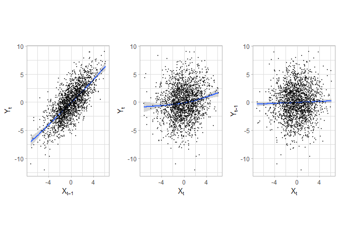
set.seed(20180108 + 1)

shannon_te <- transfer_entropy(x = x, y = y)
#> Shannon's entropy on 8 cores with 100 shuffles.
#>   x and y have length 2000 (0 NAs removed)
#>   [calculate] X->Y transfer entropy
#>   [calculate] Y->X transfer entropy
#>   [bootstrap] 300 times
#> Done - Total time 4.2 seconds

shannon_te
#> Shannon Transfer Entropy Results:
#> -----------------------------------------------------------
#> Direction        TE   Eff. TE  Std.Err.   p-value    sig
#> -----------------------------------------------------------
#>      X->Y    0.1245    0.1210    0.0014    0.0000    ***
#>      Y->X    0.0020    0.0000    0.0014    0.8467
#> -----------------------------------------------------------
#> Bootstrapped TE Quantiles (300 replications):
#> -----------------------------------------------------------
#> Direction      0%     25%     50%     75%    100%
#> -----------------------------------------------------------
#>      X->Y  0.0005  0.0022  0.0029  0.0040  0.0083
#>      Y->X  0.0008  0.0024  0.0031  0.0041  0.0088
#> -----------------------------------------------------------
#> Number of Observations: 2000
#> -----------------------------------------------------------
#> p-values: < 0.001 '***', < 0.01 '**', < 0.05 '*', < 0.1 '.'

summary(shannon_te)
#> Shannon's Transfer Entropy
#>
#> Coefficients:
#>             te       ete     se p-value
#> X->Y 0.1244709 0.1210119 0.0014  <2e-16 ***
#> Y->X 0.0020383 0.0000000 0.0014  0.8467
#> ---
#> Signif. codes:  0 '***' 0.001 '**' 0.01 '*' 0.05 '.' 0.1 ' ' 1
#>
#> Bootstrapped TE Quantiles (300 replications):
#> Direction      0%     25%     50%     75%    100%
#>      X->Y  0.0005  0.0022  0.0029  0.0040  0.0083
#>      Y->X  0.0008  0.0024  0.0031  0.0041  0.0088
#>
#> Number of Observations: 2000
Alternatively, you can calculate only the transfer entropy or the effective transfer entropy with
calc_te(x, y)
#> [1] 0.1244709
calc_te(y, x)
#> [1] 0.002038284

calc_ete(x, y)
#> [1] 0.1213265
calc_ete(y, x)
#> [1] 0set.seed(20180108 + 1)
renyi_te <- transfer_entropy(x = x, y = y, entropy = "renyi", q = 0.5)
#> Renyi's entropy on 8 cores with 100 shuffles.
#> x and y have length 2000 (0 NAs removed)
#> [calculate] X->Y transfer entropy
#> [calculate] Y->X transfer entropy
#> [bootstrap] 300 times
#> Done - Total time 3.62 seconds
renyi_te
#> Renyi Transfer Entropy Results:
#> -----------------------------------------------------------
#> Direction TE Eff. TE Std.Err. p-value sig
#> -----------------------------------------------------------
#> X->Y 0.0852 0.0393 0.0217 0.0300 *
#> Y->X 0.0276 -0.0139 0.0226 0.7233
#> -----------------------------------------------------------
#> Bootstrapped TE Quantiles (300 replications):
#> -----------------------------------------------------------
#> Direction 0% 25% 50% 75% 100%
#> -----------------------------------------------------------
#> X->Y -0.0094 0.0273 0.0404 0.0557 0.1132
#> Y->X -0.0358 0.0266 0.0421 0.0576 0.1141
#> -----------------------------------------------------------
#> Number of Observations: 2000
#> Q: 0.5
#> -----------------------------------------------------------
#> p-values: < 0.001 '***', < 0.01 '**', < 0.05 '*', < 0.1 '.'
calc_te(x, y, entropy = "renyi", q = 0.5)
#> [1] 0.08515726
calc_te(y, x, entropy = "renyi", q = 0.5)
#> [1] 0.02758021
calc_ete(x, y, entropy = "renyi", q = 0.5)
#> [1] 0.04393078
calc_ete(y, x, entropy = "renyi", q = 0.5)
#> [1] -0.01612456quiet = TRUETo disable the verbosity of a function you can use the argument
quiet. Note that we have set nboot = 0 as we
don’t need bootstrapped quantiles for this example.
te <- transfer_entropy(x, y, nboot = 0, quiet = T)

te
#> Shannon Transfer Entropy Results:
#> -----------------------------------------------------------
#> Direction        TE   Eff. TE  Std.Err.   p-value    sig
#> -----------------------------------------------------------
#>      X->Y    0.1245    0.1212        NA        NA
#>      Y->X    0.0020    0.0000        NA        NA
#> -----------------------------------------------------------
#> For calculation of standard errors and p-values set nboot > 0
#> -----------------------------------------------------------
#> Number of Observations: 2000
#> -----------------------------------------------------------
#> p-values: < 0.001 '***', < 0.01 '**', < 0.05 '*', < 0.1 '.'
If you want to disable feedback from transfer_entropy
functions, you can do so by using set_quiet(TRUE)
set_quiet(TRUE)
te <- transfer_entropy(x, y, nboot = 0)

te
#> Shannon Transfer Entropy Results:
#> -----------------------------------------------------------
#> Direction        TE   Eff. TE  Std.Err.   p-value    sig
#> -----------------------------------------------------------
#>      X->Y    0.1245    0.1211        NA        NA
#>      Y->X    0.0020    0.0000        NA        NA
#> -----------------------------------------------------------
#> For calculation of standard errors and p-values set nboot > 0
#> -----------------------------------------------------------
#> Number of Observations: 2000
#> -----------------------------------------------------------
#> p-values: < 0.001 '***', < 0.01 '**', < 0.05 '*', < 0.1 '.'

# revert back with
set_quiet(FALSE)

te <- transfer_entropy(x, y, nboot = 0)
#> Shannon's entropy on 8 cores with 100 shuffles.
#>   x and y have length 2000 (0 NAs removed)
#>   [calculate] X->Y transfer entropy
#>   [calculate] Y->X transfer entropy
#> Done - Total time 0.13 secondsUsing the future package and its plans we
can execute all computations in parallel like so
library(future)
plan(multisession)
te <- transfer_entropy(x, y, nboot = 100)
#> Shannon's entropy on 8 cores with 100 shuffles.
#>   x and y have length 2000 (0 NAs removed)
#>   [calculate] X->Y transfer entropy
#>   [calculate] Y->X transfer entropy
#>   [bootstrap] 100 times
#> Done - Total time 1.92 seconds

# revert to sequential mode
plan(sequential)
te <- transfer_entropy(x, y, nboot = 100)
#> Shannon's entropy on 1 core with 100 shuffles.
#>   x and y have length 2000 (0 NAs removed)
#>   [calculate] X->Y transfer entropy
#>   [calculate] Y->X transfer entropy
#>   [bootstrap] 100 times
#> Done - Total time 4.08 seconds

# close multisession, see also ?plan
plan(sequential)