![]()
RCTrep is an R package to validate methods for
conditional average treatment effect (CATE) estimation
using real-world data (RWD). Validation of methods for
treatment effect estimation using RWD is challenging because we do not
observe the true treatment effect for each individual  - a fundamental
problem of causal inference - hence we can only
estimate treatment effect using observed data. Randomized control trial
(RCT) assigns individuals to treatment
- a fundamental
problem of causal inference - hence we can only
estimate treatment effect using observed data. Randomized control trial
(RCT) assigns individuals to treatment
or control groups
with known
probability
 , hence two groups are balanced in terms of observed and unobserved
covariates. The difference in outcomes between groups can be merely
attributed to realization of treatment
, hence two groups are balanced in terms of observed and unobserved
covariates. The difference in outcomes between groups can be merely
attributed to realization of treatment
, and hence the
treatment effect is the simple difference in means of outcomes and is
unbiased given identification assumption holds. However, in case we
don’t know the true probability
in RWD, without knowing the ground truth,
how can we validate the methods for treatment effect
estimation?
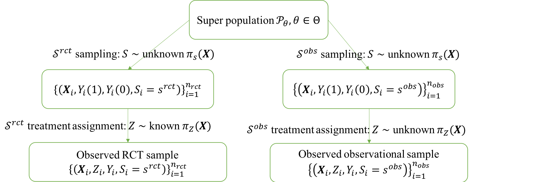
RCTrep is an R package to enable easy validation of various methods for treatment effect estimation using RWD by comparison to RCT data. We identify under which conditions the estimate from RCT can be regarded as the ground truth for methods validation using RWD. We assume the RWD and RCT data are two random samples from a, potentially different, population, and hence allow for a valid comparison of estimates of treatment effect between two samples after population composition is controlled for. We refer users to RCTrep vignettes for theoretical elaboration, in which we illustrate why estimates from RCT can be assumed as ground truth and how to use the estimates as the surrogate of the ground truth of RWD from the view of treatment assignment mechanism and sampling mechansim. We provide an diagram to show how RCT data and RWD differ in two mechanisms in the following figure:
We consider a set of candidate treatment effect estimators  , where
  , hence
  is an estimator of
conditional average treatment effect of population with characteristics
is an estimator of
conditional average treatment effect of population with characteristics
 . We provide
the package that makes it easy to try out various estimators
. We provide
the package that makes it easy to try out various estimators  and select the best
one using the following evaluation metric:
and select the best
one using the following evaluation metric:

where  is an
unbiased estimate of the average treatment effect derived from the RCT
data,
is an
unbiased estimate of the average treatment effect derived from the RCT
data,  and
and  are the empirical
density of
are the empirical
density of  in RCT data and RWD,
  is a weight for individuals in RWD with
characteristics . Hence the weighted distribution of covariates in RWD
and distribution of covariates in the RCT data are balanced. We compute
is a weight for individuals in RWD with
characteristics . Hence the weighted distribution of covariates in RWD
and distribution of covariates in the RCT data are balanced. We compute
 on
population and
sub-population levels.
on
population and
sub-population levels.
The package use R6 Object-oriented programming system. We provide an overview of implementation of RCTrep in the following figure:
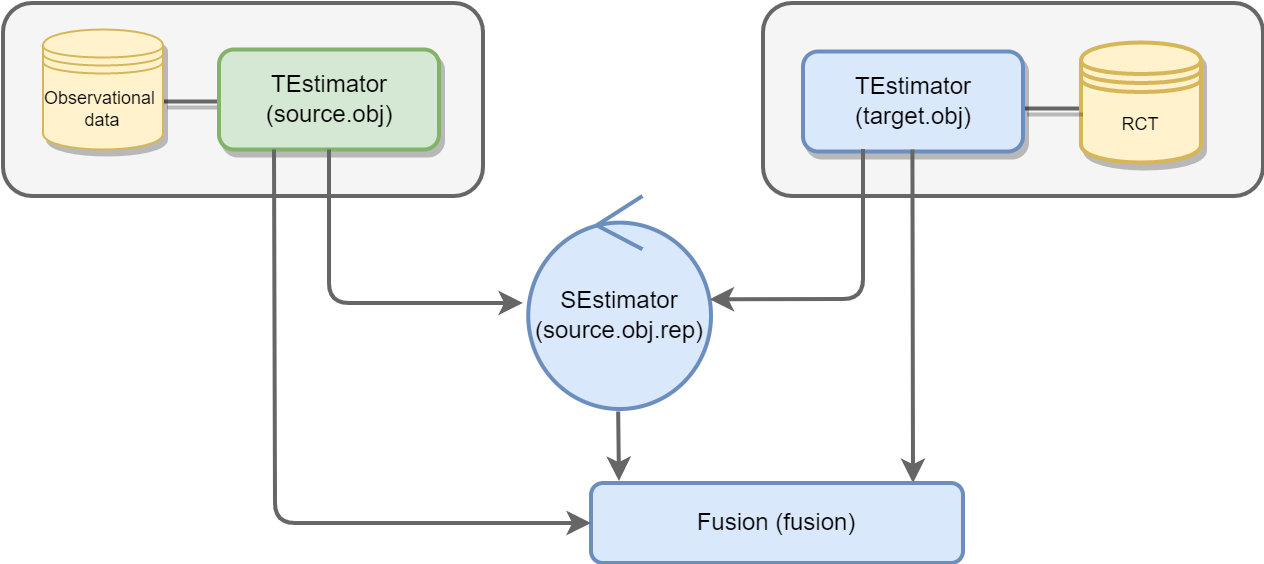
RCTrep provides two core classes, namely, TEstimator and SEstimator, which are responsible for adjusting the treatment assignment mechanism and the sampling mechanism respectively.
TEstimator has three subclasses for adjusting the treatment assignment mechanism, namely,
SEstimator has three subclasses for adjusting the sampling mechanism, namely,
Users can specify modeling approaches for sampling score, propensity
score, outcome regression, and distance measure, etc. Two
objects instantiated using RWD and experimental RCT data
communicate within the object of the class SEstimator, sharing
either unit-level data” or aggregated
data for computing the weights .
Summary R6 class Summary combines estimates from an object of class TEstimate and/or an object of class SEstimate, and plots and evaluates estimates of average treatment effect and heterogeneous treatment effect. The number of objects of class TEstimator or SEstimator passed to its constructor is not limited.
The package can also generate synthetic RCT data based on meta data from publications (point estimate and interval estimate of average treatment effect, conditional average treatment effect conditioning on univariate variable, and univariate distribution).
You can install the development version from GitHub with:
# install.packages("devtools")
devtools::install_github("duolajiang/RCTrep")
We will realease the package to CRAN soon.
We demonstrate the simple usage of RCTrep to validate methods for treatment effect estimation. We use G-computation to adjust for the treatment assignment mechanism - the method using RWD to validate. We use exact matching to balance covariates between RWD and RCT data, and obtain the weighted estimates of treatment effect using RWD. Then we can implement the fair comparison between weighted estimates using RWD and unbiased estimate using experimental data. Variables that may confound causal association between treatment and outcome, and variables that may lead to supurious association between sampling and outcomes still need careful investigation and identification.
This step is to identify the variable set outcome_predictors that confound causal relation between treatment and outcome, and the variable set selection_predictors that can induce spurious difference in estimates between RWD and RCT data.
library(RCTrep)
source.data <- RCTrep::source.data
target.data <- RCTrep::target.data

vars_name <- list(outcome_predictors=c("x1","x2","x3","x4","x5","x6"),
                  treatment_name=c('z'),
                  outcome_name=c('y')
)
selection_predictors <- c("x1","x2","x3","x4","x5","x6")source.obj <- TEstimator_wrapper(
Estimator = "G_computation",
data = source.data,
name = "RWD",
vars_name = vars_name,
outcome_method = "glm",
outcome_formula = y ~ x1 + x2 + x3 + z + z:x1 + z:x2 +z:x3+ z:x6,
data.public = TRUE
)
#> y ~ x1 + x2 + x3 + z + z:x1 + z:x2 + z:x3 + z:x6
target.obj <- TEstimator_wrapper(
Estimator = "Crude",
data = target.data,
name = "RCT",
vars_name = vars_name,
data.public = TRUE,
isTrial = TRUE
)# step2.2: Estimation of weighted treatment effect
source.obj.rep <- SEstimator_wrapper(Estimator="Exact",
target.obj=target.obj,
source.obj=source.obj,
selection_predictors=selection_predictors)
source.obj.rep$EstimateRep(stratification = c("x1","x3","x4","x5"))This step diagnoses model assumption for G-computation (covariats balance for IPW), treatment overlap assumption, outcome overlap assumption, and sampling overlap assumption.
source.obj$diagnosis_t_ignorability()
#> $residuals.overall
#> [1] 2.214633e-14
#>
#> $residuals.subgroups
#>    x1 x2 x3 x4 x5 x6 sample.size     res.mean     res.se       msr       sesr
#> 1   0  0  0  0  0  0           8 -0.033159812 0.28630939 0.5749111 0.25909656
#> 2   0  0  0  0  0  1          31 -0.099669263 0.15500392 0.7307204 0.16986746
#> 3   0  0  0  0  1  0          16 -0.291784223 0.22392759 0.8372915 0.33709962
#> 4   0  0  0  0  1  1          68 -0.081493792 0.10890826 0.8013288 0.12627815
#> 5   0  0  0  1  0  0          29  0.289766947 0.18601148 1.0527725 0.28109093
#> 6   0  0  0  1  0  1         122 -0.018623426 0.09563139 1.1069356 0.10495348
#> 7   0  0  0  1  1  1         297 -0.039424153 0.05472699 0.8880872 0.07021318
#> 8   0  0  1  0  0  0          27  0.359416934 0.23566150 1.5731255 0.27345679
#> 9   0  0  1  0  0  1         116 -0.064430174 0.10341172 1.2339593 0.14397971
#> 10  0  0  1  0  1  0          73  0.122384056 0.11547447 0.9750512 0.17221696
#> 11  0  0  1  1  0  0         140 -0.103108837 0.08108053 0.9244247 0.09551924
#> 12  0  0  1  1  1  0         259  0.042947650 0.06087029 0.9577841 0.09134774
#> 13  0  1  0  0  0  1           7 -0.536943485 0.34724241 1.0117720 0.69268561
#> 14  0  1  0  0  1  0           5 -0.138659594 0.21350193 0.2015588 0.10876393
#> 15  0  1  0  0  1  1          16 -0.044121152 0.27092416 1.1029452 0.37762497
#> 16  0  1  0  1  0  1          33 -0.029399192 0.16582744 0.8808240 0.32867335
#> 17  0  1  0  1  1  0          15  0.225047363 0.28999923 1.2280401 0.50759032
#> 18  0  1  0  1  1  1          79  0.111122348 0.11518856 1.0472837 0.14102420
#> 19  0  1  1  0  0  0          10 -0.489153001 0.28166251 0.9532746 0.23392786
#> 20  0  1  1  0  0  1          28  0.043123603 0.20235159 1.1074062 0.29713360
#> 21  0  1  1  0  1  0          19  0.003265044 0.27119153 1.3238179 0.31297388
#> 22  0  1  1  0  1  1          72  0.002178221 0.10858861 0.8372002 0.15777598
#> 23  0  1  1  1  0  0          35  0.170865832 0.13459768 0.6451573 0.14548423
#> 24  0  1  1  1  0  1         125 -0.056121898 0.09058246 1.0205923 0.15850343
#> 25  0  1  1  1  1  0          65  0.040177469 0.12293937 0.9689158 0.23001168
#> 26  0  1  1  1  1  1         296  0.024164125 0.05184835 0.7936179 0.06180646
#> 27  1  0  0  0  0  0           2  1.020056964 1.04248503 2.1272913 2.12678823
#> 28  1  0  0  0  1  0           4  0.590859805 0.43729538 0.9227971 0.51590407
#> 29  1  0  0  0  1  1          22 -0.027696594 0.18169792 0.6940639 0.14754895
#> 30  1  0  0  1  0  0          11  0.249437181 0.31263135 1.0396025 0.31885782
#> 31  1  0  0  1  0  1          36  0.220385980 0.17795769 1.1569829 0.19544718
#> 32  1  0  0  1  1  0          16  0.048570074 0.19875700 0.5949242 0.15698698
#> 33  1  0  1  0  0  0           9  0.197302831 0.31820751 0.8489766 0.40225460
#> 34  1  0  1  0  0  1          32 -0.045410644 0.18378995 1.0492033 0.18998055
#> 35  1  0  1  0  1  0          19  0.092662797 0.25283001 1.1592007 0.44746032
#> 36  1  0  1  0  1  1          71  0.043913387 0.12107083 1.0279986 0.16060356
#> 37  1  0  1  1  0  0          32  0.179626509 0.14713726 0.7033962 0.15161745
#> 38  1  0  1  1  0  1         121 -0.118212578 0.08039760 0.7896270 0.09712507
#> 39  1  0  1  1  1  0          67 -0.009015888 0.13323385 1.1716644 0.21134724
#> 40  1  1  0  0  0  1           3 -0.801041824 0.30720451 0.8304172 0.58650330
#> 41  1  1  0  1  0  0           2  0.116839187 0.44234613 0.2093215 0.10336672
#> 42  1  1  0  1  0  1           9  0.061176434 0.40000603 1.2837812 0.60733013
#> 43  1  1  0  1  1  0           4  0.023281191 0.34205505 0.3515470 0.20537435
#> 44  1  1  0  1  1  1          20 -0.030336997 0.26684840 1.3538736 0.39312787
#> 45  1  1  1  0  0  1          12  0.002671423 0.15873990 0.2771891 0.11673024
#> 46  1  1  1  0  1  0           5 -0.260903445 0.54680276 1.2640436 0.56667606
#> 47  1  1  1  0  1  1          14 -0.231240962 0.30847904 1.2905435 0.36617811
#> 48  1  1  1  1  0  0           8  0.062835422 0.18528567 0.2442638 0.11057093
#> 49  1  1  1  1  0  1          32  0.193141574 0.15858574 0.8169362 0.24339579
#> 50  1  1  1  1  1  0           9 -0.024257039 0.20129750 0.3247539 0.14474685
#> 51  1  1  1  1  1  1          71 -0.156520230 0.10575745 0.8074232 0.12569119
#>
#> $plot.res.mse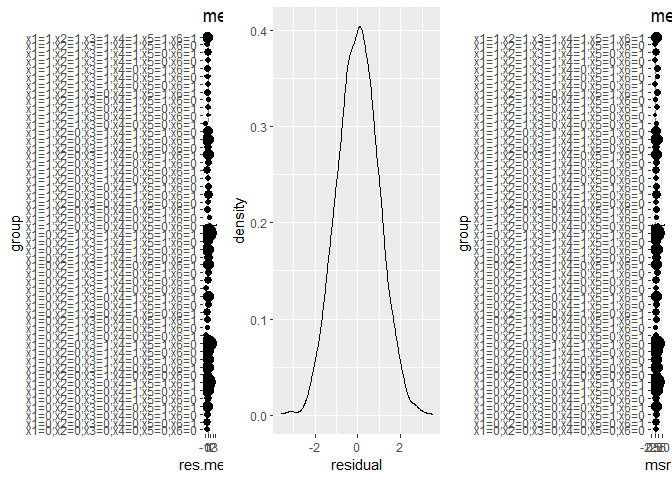
source.obj$diagnosis_t_overlap()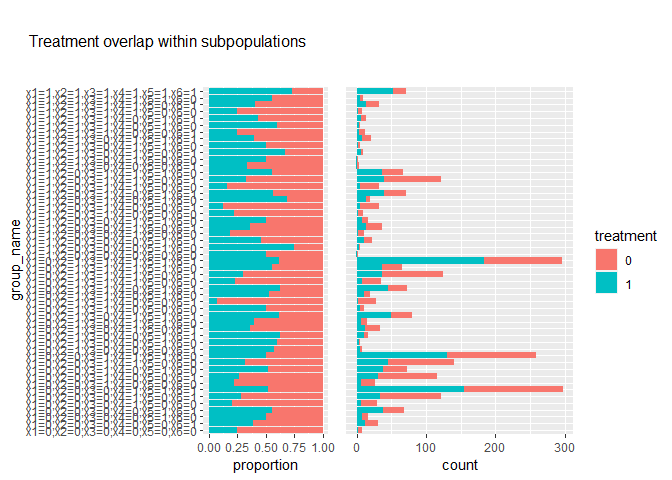
source.obj.rep$diagnosis_s_ignorability()
#> to be continued... This function is to check if
#>               confounders_sampling are balanced between source and target object
#>               on population and sub-population levels stratified by
#>               stratificaiton and stratification_joint.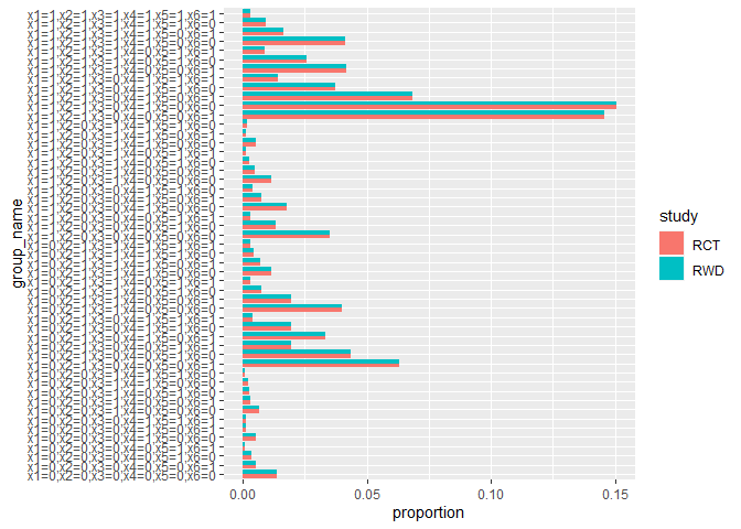
source.obj.rep$diagnosis_s_overlap()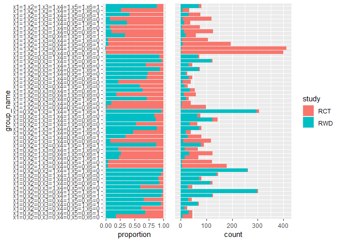
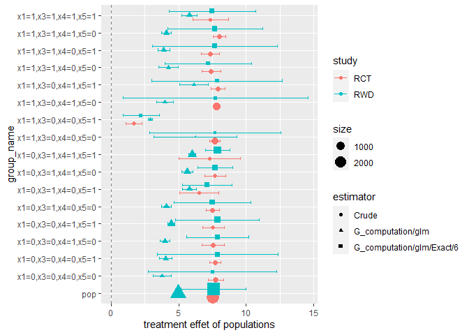
This step compare the estimates from RWD with those from RCT data, and validate difference methods using RWD.
fusion <- Fusion$new(target.obj,
                     source.obj,
                     source.obj.rep)
fusion$evaluate()
#> # A tibble: 34 x 7
#> # Groups:   group_name [17]
#>    group_name          estimator             size     mse len_ci agg.est agg.reg
#>    <chr>               <chr>                <dbl>   <dbl>  <dbl> <lgl>   <lgl>
#>  1 pop                 G_computation/glm/E~  2622 9.8 e-2  4.83  TRUE    TRUE
#>  2 pop                 G_computation/glm     2622 6.66e+2  0.239 FALSE   TRUE
#>  3 x1=0,x3=0,x4=0,x5=0 G_computation/glm/E~    46 5.58e+0  9.53  TRUE    TRUE
#>  4 x1=0,x3=0,x4=0,x5=0 G_computation/glm       46 1.58e+3  1.33  FALSE   TRUE
#>  5 x1=0,x3=0,x4=0,x5=1 G_computation/glm/E~   105 3.55e+0  8.94  TRUE    TRUE
#>  6 x1=0,x3=0,x4=0,x5=1 G_computation/glm      105 1.35e+3  0.938 FALSE   TRUE
#>  7 x1=0,x3=0,x4=1,x5=0 G_computation/glm/E~   184 1.21e+1  4.64  TRUE    TRUE
#>  8 x1=0,x3=0,x4=1,x5=0 G_computation/glm      184 1.28e+3  0.707 FALSE   TRUE
#>  9 x1=0,x3=0,x4=1,x5=1 G_computation/glm/E~   391 9.47e+0  6.21  TRUE    TRUE
#> 10 x1=0,x3=0,x4=1,x5=1 G_computation/glm      391 9.68e+2  0.502 FALSE   TRUE
#> # i 24 more rows
fusion$plot()