![]()
![]()
![]()
The goal of PointedSDMs is to simplify the construction of integrated species distribution models (ISDMs) for large collections of heterogeneous data. It does so by building wrapper functions around inlabru, which uses the INLA methodology to estimate a class of latent Gaussian models.
You can install the development version of PointedSDMs from GitHub with:
# install.packages("devtools")
devtools::install_github("PhilipMostert/PointedSDMs")
or directly through CRAN using:
install.packages('PointedSDMs')PointedSDMs includes a selection of functions used to streamline the construction of ISDMs as well and perform model cross-validation. The core functions of the package are:
| Function name | Function description |
|---|---|
startISDM() |
Initialize and specify the components used in the integrated model. |
startSpecies() |
Initialize and specify the components used in the multi-species integrated model. |
blockedCV() |
Perform spatial blocked cross-validation. |
fitISDM() |
Estimate and preform inference on the integrated model. |
datasetOut() |
Perform dataset-out cross-validation, which calculates the impact individual datasets have on the full model. |
The function intModel() produces an R6 object, and as a result there
are various slot functions available to further specify the
components of the model. These slot functions include:
intModel() slot function |
Function description |
|---|---|
`.$help()` |
Show documentation for each of the slot functions. |
`.$plot()` |
Used to create a plot of the available data. The output of this
function is an object of class gg. |
`.$addBias()` |
Add an additional spatial field to a dataset to account for sampling bias in unstructured datasets. |
`.$updateFormula()` |
Used to update a formula for a process. The idea is to start specify
the full model with startISDM(), and then thin components
per dataset with this function. |
`.$updateComponents()` |
Change or add new components used by inlabru in the integrated model. |
`.$priorsFixed()` |
Change the specification of the prior distribution for the fixed effects in the model. |
`.$specifySpatial()` |
Specify the spatial field in the model using penalizing complexity (PC) priors. |
`.$spatialBlock()` |
Used to specify how the points are spatially blocked. Spatial
cross-validation is subsequently performed using
blockedCV(). |
`.$addSamplers()` |
Function to add an integration domain for the PO datasets. |
`.$specifyRandom()` |
Specify the priors for the random effects in the model. |
`.$changeLink()` |
Change the link function of a process. |
This is a basic example which shows you how to specify and run an integrated model, using three disparate datasets containing locations of the solitary tinamou (Tinamus solitarius).
library(PointedSDMs)
library(ggplot2)
library(terra)
bru_options_set(inla.mode = "experimental")

#Load data in

data("SolitaryTinamou")

projection <- "+proj=longlat +ellps=WGS84"

species <- SolitaryTinamou$datasets

covariates <- terra::rast(system.file('extdata/SolitaryTinamouCovariates.tif',
                                      package = "PointedSDMs"))

mesh <- SolitaryTinamou$mesh
Setting up the model is done easily with startISDM(),
where we specify the required components of the model:
#Specify model -- here we run a model with one spatial covariate and a shared spatial field

model <- startISDM(species, spatialCovariates = covariates,
                 Projection = projection, Mesh = mesh, responsePA = 'Present')
We can also make a quick plot of where the species are located using
`.$plot()`:
region <- SolitaryTinamou$region

model$plot(Boundary = FALSE) +
  geom_sf(data = st_boundary(region))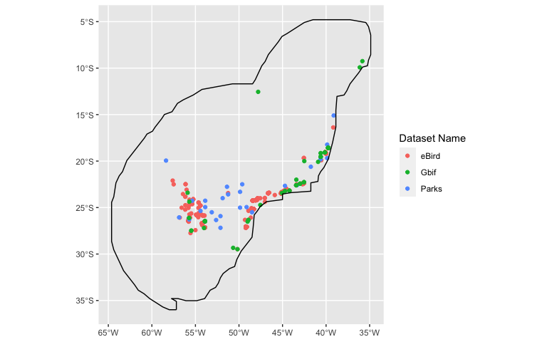
To improve stability, we specify priors for the intercepts of the
model using `.$priorsFixed()`
model$priorsFixed(Effect = 'Intercept',
                  mean.linear = 0,
                  prec.linear = 1)
And PC priors for the spatial field using
`.$specifySpatial()`:
model$specifySpatial(sharedSpatial = TRUE,
                     prior.range = c(0.2, 0.1),
                     prior.sigma = c(0.1, 0.1))
We can then estimate the parameters in the model using the
fitISDM() function:
modelRun <- fitISDM(model, options = list(control.inla =
list(int.strategy = 'eb'),
safe = TRUE))
summary(modelRun)
#> Summary of 'modISDM' object:
#>
#> inlabru version: 2.12.0
#> INLA version: 24.06.27
#>
#> Types of data modelled:
#>
#> eBird Present only
#> Parks Present absence
#> Gbif Present only
#> Time used:
#> Pre = 1.16, Running = 21.3, Post = 0.274, Total = 22.7
#> Fixed effects:
#> mean sd 0.025quant 0.5quant 0.975quant mode kld
#> Forest 0.054 0.006 0.042 0.054 0.066 0.054 0
#> NPP 0.000 0.000 0.000 0.000 0.000 0.000 0
#> Altitude -0.002 0.001 -0.003 -0.002 -0.001 -0.002 0
#> eBird_intercept -5.419 0.435 -6.271 -5.419 -4.567 -5.419 0
#> Parks_intercept -4.783 0.485 -5.734 -4.783 -3.832 -4.783 0
#> Gbif_intercept -6.128 0.412 -6.936 -6.128 -5.320 -6.128 0
#>
#> Random effects:
#> Name Model
#> eBird_spatial SPDE2 model
#> Parks_spatial Copy
#> Gbif_spatial Copy
#>
#> Model hyperparameters:
#> mean sd 0.025quant 0.5quant 0.975quant mode
#> Range for eBird_spatial 3.615 0.912 2.460 3.421 5.946 2.92
#> Stdev for eBird_spatial 2.514 0.427 1.924 2.438 3.567 2.21
#> Beta for Parks_spatial 0.137 0.100 -0.043 0.133 0.348 0.11
#> Beta for Gbif_spatial 0.714 0.067 0.585 0.713 0.848 0.71
#>
#> Deviance Information Criterion (DIC) ...............: 259.79
#> Deviance Information Criterion (DIC, saturated) ....: 253.61
#> Effective number of parameters .....................: -840.82
#>
#> Watanabe-Akaike information criterion (WAIC) ...: 2441.50
#> Effective number of parameters .................: 686.08
#>
#> Marginal log-Likelihood: -1330.87
#> is computed
#> Posterior summaries for the linear predictor and the fitted values are computed
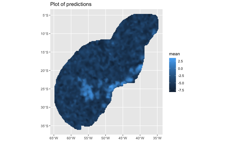
#> (Posterior marginals needs also 'control.compute=list(return.marginals.predictor=TRUE)')PointedSDMs also includes generic predict and plot functions:
predictions <- predict(modelRun, mesh = mesh,
                       mask = region,
                       spatial = TRUE,
                       fun = 'linear')

plot(predictions, variable = c('mean', 'sd'))