PDtoolkit provides collection of tools for probability
of default (PD) rating model development and validation. Keeping in
mind the fact that model development is highly iterative and repetitive
process, having standardized and automated tools for this purpose is of
the utmost importance for analysts. The main goal of this package is to
cover the most common steps of PD model development. As additional
contribution we attempted to add some functionalities which at the
moment of the package development were not presented in R
package ecosystem in area of credit risk modeling. The package available
functionalities are those that refer to univariate, bivariate,
multivariate analysis, calibration and validation. Along with
accompanied monobin and monobinShiny packages,
PDtoolkit provides functions which are suitable for
different data transformation and modeling tasks such as: imputations,
monotonic binning of numeric risk factors, binning of categorical risk
factors, weights of evidence (WoE) and information value (IV)
calculations, WoE coding (replacement of risk factors’ modalities with
WoE values), risk factor clustering, area under curve (AUC) calculation
and others. Beside mentioned features, package provides set of
validation functions for testing homogeneity, heterogeneity,
discriminatory and predictive power of the model.
The following case study shows the usage of PDtoolkit
package. The study is based on publicly available German credit data set
which is available and downloaded from this link, but also
distributed along with PDtoolkit package under the data
frame loans. Presented examples are simplified, but yet
realistic, version of the PD model development and validation. In the
first row, simplification is assumed in final model selection, master
scale creation, calibration and some validation steps, whereas in
practice we usually have highly iterative process with couple of
available options. Anyhow, this does not diminish the practical value of
the presented examples. So, let’s start with a concrete case study.
First, we will import the libraries needed for the following examples.
library(PDtoolkit)
library(monobin)
library(rpart)
If the packages are not already installed, run the following code
before the library import
install.packages(c("PDtoolkit", "monobin", "rpart")) in
order to install it from the CRAN, while
devtools::install_github("andrija-djurovic/PDtoolkit") to
install development version.
Then, let’s import and inspect the structure of the modeling data set
- loans.
data(loans)
str(loans)
## 'data.frame': 1000 obs. of 21 variables:
## $ Creditability : num 0 0 0 0 0 0 0 0 0 0 ...
## $ Account Balance : chr "1" "1" "2" "1" ...
## $ Duration of Credit (month) : num 18 9 12 12 12 10 8 6 18 24 ...
## $ Payment Status of Previous Credit: chr "4" "4" "2" "4" ...
## $ Purpose : chr "2" "0" "9" "0" ...
## $ Credit Amount : num 1049 2799 841 2122 2171 ...
## $ Value Savings/Stocks : chr "1" "1" "2" "1" ...
## $ Length of current employment : chr "2" "3" "4" "3" ...
## $ Instalment per cent : chr "4" "2" "2" "3" ...
## $ Sex & Marital Status : chr "2" "3" "2" "3" ...
## $ Guarantors : chr "1" "1" "1" "1" ...
## $ Duration in Current address : chr "4" "2" "4" "2" ...
## $ Most valuable available asset : chr "2" "1" "1" "1" ...
## $ Age (years) : num 21 36 23 39 38 48 39 40 65 23 ...
## $ Concurrent Credits : chr "3" "3" "3" "3" ...
## $ Type of apartment : chr "1" "1" "1" "1" ...
## $ No of Credits at this Bank : chr "1" "2" "1" "2" ...
## $ Occupation : chr "3" "3" "2" "2" ...
## $ No of dependents : chr "1" "2" "1" "2" ...
## $ Telephone : chr "1" "1" "1" "1" ...
## $ Foreign Worker : chr "1" "1" "1" "2" ...Note that variable (column) names have some special characters which
is not usually considered as good practice in real studies, but for this
example we will use it as provided originally in data source.
Additionally, in order to present all functionalities of the
PDtoolkit package, we will slightly modify modeling data
set inserting some missing values for certain variables as given
below:
loans$"Credit Amount"[1:10] <- NA
loans$"Age (years)"[30:50] <- NA
loans$"Purpose"[800:820] <- NA
Usually the first step in model development is the univariate
analysis. For this purpose we will use univariate function
from the PDtoolkit package:
univariate(db = loans)## rf rf.type bin.type bin cnt pct
## 1 Creditability numeric complete cases complete cases 1000 1.000
## 2 Account Balance character complete cases complete cases 1000 1.000
## 3 Duration of Credit (month) numeric complete cases complete cases 1000 1.000
## 4 Payment Status of Previous Credit character complete cases complete cases 1000 1.000
## 5 Purpose character special cases special cases 21 0.021
## 6 Purpose character complete cases complete cases 979 0.979
## 7 Credit Amount numeric special cases special cases 10 0.010
## 8 Credit Amount numeric complete cases complete cases 990 0.990
## 9 Value Savings/Stocks character complete cases complete cases 1000 1.000
## 10 Length of current employment character complete cases complete cases 1000 1.000
## 11 Instalment per cent character complete cases complete cases 1000 1.000
## 12 Sex & Marital Status character complete cases complete cases 1000 1.000
## 13 Guarantors character complete cases complete cases 1000 1.000
## 14 Duration in Current address character complete cases complete cases 1000 1.000
## 15 Most valuable available asset character complete cases complete cases 1000 1.000
## 16 Age (years) numeric special cases special cases 21 0.021
## 17 Age (years) numeric complete cases complete cases 979 0.979
## 18 Concurrent Credits character complete cases complete cases 1000 1.000
## 19 Type of apartment character complete cases complete cases 1000 1.000
## 20 No of Credits at this Bank character complete cases complete cases 1000 1.000
## 21 Occupation character complete cases complete cases 1000 1.000
## 22 No of dependents character complete cases complete cases 1000 1.000
## 23 Telephone character complete cases complete cases 1000 1.000
## 24 Foreign Worker character complete cases complete cases 1000 1.000
## cnt.unique min p1 p5 p25 p50 avg avg.se p75 p95 p99
## 1 2 0 0.00 0.00 0.00 0 0.30000 0.01449863 1.00 1.0 1.00
## 2 4 NA NA NA NA NA NA NA NA NA NA
## 3 33 4 6.00 6.00 12.00 18 20.90300 0.38133320 24.00 48.0 60.00
## 4 5 NA NA NA NA NA NA NA NA NA NA
## 5 1 NA NA NA NA NA NA NA NA NA NA
## 6 10 NA NA NA NA NA NA NA NA NA NA
## 7 1 Inf NA NA NA NA NaN NA NA NA NA
## 8 915 250 424.13 708.45 1371.25 2324 3283.24242 90.03256824 3978.25 9219.7 14194.29
## 9 5 NA NA NA NA NA NA NA NA NA NA
## 10 5 NA NA NA NA NA NA NA NA NA NA
## 11 4 NA NA NA NA NA NA NA NA NA NA
## 12 4 NA NA NA NA NA NA NA NA NA NA
## 13 3 NA NA NA NA NA NA NA NA NA NA
## 14 4 NA NA NA NA NA NA NA NA NA NA
## 15 4 NA NA NA NA NA NA NA NA NA NA
## 16 1 Inf NA NA NA NA NaN NA NA NA NA
## 17 53 19 20.00 22.00 27.00 33 35.52605 0.36315861 42.00 60.0 67.22
## 18 3 NA NA NA NA NA NA NA NA NA NA
## 19 3 NA NA NA NA NA NA NA NA NA NA
## 20 4 NA NA NA NA NA NA NA NA NA NA
## 21 4 NA NA NA NA NA NA NA NA NA NA
## 22 2 NA NA NA NA NA NA NA NA NA NA
## 23 2 NA NA NA NA NA NA NA NA NA NA
## 24 2 NA NA NA NA NA NA NA NA NA NA
## max neg pos cnt.outliers sc.ind
## 1 1 0 300 0 0
## 2 NA NA NA NA 0
## 3 72 0 1000 70 0
## 4 NA NA NA NA 0
## 5 NA NA NA NA 0
## 6 NA NA NA NA 0
## 7 -Inf NA NA 0 0
## 8 18424 0 990 72 0
## 9 NA NA NA NA 0
## 10 NA NA NA NA 0
## 11 NA NA NA NA 0
## 12 NA NA NA NA 0
## 13 NA NA NA NA 0
## 14 NA NA NA NA 0
## 15 NA NA NA NA 0
## 16 -Inf NA NA 0 0
## 17 75 0 979 23 0
## 18 NA NA NA NA 0
## 19 NA NA NA NA 0
## 20 NA NA NA NA 0
## 21 NA NA NA NA 0
## 22 NA NA NA NA 0
## 23 NA NA NA NA 0
## 24 NA NA NA NA 0Based on the results we can see that univariate treats
differently so-called special and complete cases. For result details and
additional arguments of univariate function check help page
?univariate.
From the structure and univariate results, we conclude that there are
four numeric variables, while the rest are categorical. One of the
numeric variables Creditability presents binary indicator
(0/1) of default status which will serve as our dependent variable for
PD model development. The rest of the variables present potential risk
factors for the PD model. Additionally, we see that some risk factors
(Purpose, Credit Amount,
Age (years)) have certain share of special cases and that
for numeric risk factors potential outliers are identified. Sometimes,
analysts want to impute certain values instead of special cases (usually
missing values) as well as for potential outliers. Without going too
much into deeper analysis for this case study we can perform imputations
using two functions from PDtoolkitpackage:
imp.sc for special cases and imp.outliers for
outliers.
#imputation for special cases for risk factors "Credit Amount", "Purpose"
imp.sc.res <- imp.sc(db = loans[, c("Credit Amount", "Purpose")],
               method.num = "automatic",
               p.val = 0.05)
names(imp.sc.res)
## [1] "db" "report"#new risk factors with imputed values
head(imp.sc.res[[1]])## Credit Amount Purpose
## 1 2324 2
## 2 2324 0
## 3 2324 9
## 4 2324 0
## 5 2324 0
## 6 2324 0#imputation report
imp.sc.res[[2]]## rf info imputation.method imputed.value imputation.num
## 1 Credit Amount Imputation completed. automatic - median 2324 10
## 2 Purpose Imputation completed. mode NA 21
## imputed.mode
## 1 <NA>
## 2 3#replace Credit Amount and Purpose with new values
loans[, c("Credit Amount", "Purpose")] <- imp.sc.res[[1]]
colSums(is.na(loans))## Creditability Account Balance
## 0 0
## Duration of Credit (month) Payment Status of Previous Credit
## 0 0
## Purpose Credit Amount
## 0 0
## Value Savings/Stocks Length of current employment
## 0 0
## Instalment per cent Sex & Marital Status
## 0 0
## Guarantors Duration in Current address
## 0 0
## Most valuable available asset Age (years)
## 0 21
## Concurrent Credits Type of apartment
## 0 0
## No of Credits at this Bank Occupation
## 0 0
## No of dependents Telephone
## 0 0
## Foreign Worker
## 0#imputation for outliers for risk factor Credit Amount
imp.out.res <- imp.outliers(db = loans[, "Credit Amount", drop = FALSE],
method = "iqr",
range = 1.5)
#new risk factors with imputed values
head(imp.out.res[[1]])## Credit Amount
## 1 2324
## 2 2324
## 3 2324
## 4 2324
## 5 2324
## 6 2324#imputation report
imp.out.res[[2]]## rf info imputation.method imputation.val.upper
## 1 Credit Amount Imputation completed. iqr 7865
## imputation.val.lower imputation.num.upper imputation.num.lower
## 1 250 73 0#replace Credit Amount with new values
loans[, "Credit Amount"] <- imp.out.res[[1]]Usually, when building PD models numeric risk factors are
discretized, so we will proceed next with that step. For the purpose of
binning the numeric risk factors, we will use one of the functions
(ndr.bin) from the monobin package. Details
about this package can be found here.
#identify numeric risk factors
num.rf <- sapply(loans, is.numeric)
num.rf <- names(num.rf)[!names(num.rf)%in%"Creditability" & num.rf]
#discretized numeric risk factors using ndr.bin from monobin package
loans[, num.rf] <- sapply(num.rf, function(x)
                  monobin::ndr.bin(x = loans[, x], y = loans[, "Creditability"])[[2]])
#check loans structure again and confirm binning was sucessful
str(loans)
## 'data.frame': 1000 obs. of 21 variables:
## $ Creditability : num 0 0 0 0 0 0 0 0 0 0 ...
## $ Account Balance : chr "1" "1" "2" "1" ...
## $ Duration of Credit (month) : chr "03 [16,45)" "02 [8,16)" "02 [8,16)" "02 [8,16)" ...
## $ Payment Status of Previous Credit: chr "4" "4" "2" "4" ...
## $ Purpose : chr "2" "0" "9" "0" ...
## $ Credit Amount : chr "01 (-Inf,3914)" "01 (-Inf,3914)" "01 (-Inf,3914)" "01 (-Inf,3914)" ...
## $ Value Savings/Stocks : chr "1" "1" "2" "1" ...
## $ Length of current employment : chr "2" "3" "4" "3" ...
## $ Instalment per cent : chr "4" "2" "2" "3" ...
## $ Sex & Marital Status : chr "2" "3" "2" "3" ...
## $ Guarantors : chr "1" "1" "1" "1" ...
## $ Duration in Current address : chr "4" "2" "4" "2" ...
## $ Most valuable available asset : chr "2" "1" "1" "1" ...
## $ Age (years) : chr "01 (-Inf,26)" "03 [35,Inf)" "01 (-Inf,26)" "03 [35,Inf)" ...
## $ Concurrent Credits : chr "3" "3" "3" "3" ...
## $ Type of apartment : chr "1" "1" "1" "1" ...
## $ No of Credits at this Bank : chr "1" "2" "1" "2" ...
## $ Occupation : chr "3" "3" "2" "2" ...
## $ No of dependents : chr "1" "2" "1" "2" ...
## $ Telephone : chr "1" "1" "1" "1" ...
## $ Foreign Worker : chr "1" "1" "1" "2" ...As we can see after the binning, all risk factors are categorical.
Now the modeling data set is ready for bivariate analysis. For that
purpose we will use the function bivariate from the
PDtoolkitpackage.
bivariate(db = loans, target = "Creditability")## $results
## rf bin no ng nb pct.o pct.g
## 1 Account Balance 1 274 139 135 0.274 0.198571429
## 2 Account Balance 2 269 164 105 0.269 0.234285714
## 3 Account Balance 3 63 49 14 0.063 0.070000000
## 4 Account Balance 4 394 348 46 0.394 0.497142857
## 5 Duration of Credit (month) 01 (-Inf,8) 87 78 9 0.087 0.111428571
## 6 Duration of Credit (month) 02 [8,16) 344 264 80 0.344 0.377142857
## 7 Duration of Credit (month) 03 [16,45) 499 328 171 0.499 0.468571429
## 8 Duration of Credit (month) 04 [45,Inf) 70 30 40 0.070 0.042857143
## 9 Payment Status of Previous Credit 0 40 15 25 0.040 0.021428571
## 10 Payment Status of Previous Credit 1 49 21 28 0.049 0.030000000
## 11 Payment Status of Previous Credit 2 530 361 169 0.530 0.515714286
## 12 Payment Status of Previous Credit 3 88 60 28 0.088 0.085714286
## 13 Payment Status of Previous Credit 4 293 243 50 0.293 0.347142857
## 14 Purpose 0 224 145 79 0.224 0.207142857
## 15 Purpose 1 102 86 16 0.102 0.122857143
## 16 Purpose 10 12 7 5 0.012 0.010000000
## 17 Purpose 2 177 123 54 0.177 0.175714286
## 18 Purpose 3 300 218 82 0.300 0.311428571
## 19 Purpose 4 12 8 4 0.012 0.011428571
## 20 Purpose 5 21 14 7 0.021 0.020000000
## 21 Purpose 6 49 28 21 0.049 0.040000000
## 22 Purpose 8 9 8 1 0.009 0.011428571
## 23 Purpose 9 94 63 31 0.094 0.090000000
## 24 Credit Amount 01 (-Inf,3914) 739 550 189 0.739 0.785714286
## 25 Credit Amount 02 [3914,Inf) 261 150 111 0.261 0.214285714
## 26 Value Savings/Stocks 1 603 386 217 0.603 0.551428571
## 27 Value Savings/Stocks 2 103 69 34 0.103 0.098571429
## 28 Value Savings/Stocks 3 63 52 11 0.063 0.074285714
## 29 Value Savings/Stocks 4 48 42 6 0.048 0.060000000
## 30 Value Savings/Stocks 5 183 151 32 0.183 0.215714286
## 31 Length of current employment 1 62 39 23 0.062 0.055714286
## 32 Length of current employment 2 172 102 70 0.172 0.145714286
## 33 Length of current employment 3 339 235 104 0.339 0.335714286
## 34 Length of current employment 4 174 135 39 0.174 0.192857143
## 35 Length of current employment 5 253 189 64 0.253 0.270000000
## 36 Instalment per cent 1 136 102 34 0.136 0.145714286
## 37 Instalment per cent 2 231 169 62 0.231 0.241428571
## 38 Instalment per cent 3 157 112 45 0.157 0.160000000
## 39 Instalment per cent 4 476 317 159 0.476 0.452857143
## 40 Sex & Marital Status 1 50 30 20 0.050 0.042857143
## 41 Sex & Marital Status 2 310 201 109 0.310 0.287142857
## 42 Sex & Marital Status 3 548 402 146 0.548 0.574285714
## 43 Sex & Marital Status 4 92 67 25 0.092 0.095714286
## 44 Guarantors 1 907 635 272 0.907 0.907142857
## 45 Guarantors 2 41 23 18 0.041 0.032857143
## 46 Guarantors 3 52 42 10 0.052 0.060000000
## 47 Duration in Current address 1 130 94 36 0.130 0.134285714
## 48 Duration in Current address 2 308 211 97 0.308 0.301428571
## 49 Duration in Current address 3 149 106 43 0.149 0.151428571
## 50 Duration in Current address 4 413 289 124 0.413 0.412857143
## 51 Most valuable available asset 1 282 222 60 0.282 0.317142857
## 52 Most valuable available asset 2 232 161 71 0.232 0.230000000
## 53 Most valuable available asset 3 332 230 102 0.332 0.328571429
## 54 Most valuable available asset 4 154 87 67 0.154 0.124285714
## 55 Age (years) 01 (-Inf,26) 187 108 79 0.187 0.154285714
## 56 Age (years) 02 [26,35) 349 238 111 0.349 0.340000000
## 57 Age (years) 03 [35,Inf) 443 335 108 0.443 0.478571429
## 58 Age (years) SC 21 19 2 0.021 0.027142857
## 59 Concurrent Credits 1 139 82 57 0.139 0.117142857
## 60 Concurrent Credits 2 47 28 19 0.047 0.040000000
## 61 Concurrent Credits 3 814 590 224 0.814 0.842857143
## 62 Type of apartment 1 179 109 70 0.179 0.155714286
## 63 Type of apartment 2 714 528 186 0.714 0.754285714
## 64 Type of apartment 3 107 63 44 0.107 0.090000000
## 65 No of Credits at this Bank 1 633 433 200 0.633 0.618571429
## 66 No of Credits at this Bank 2 333 241 92 0.333 0.344285714
## 67 No of Credits at this Bank 3 28 22 6 0.028 0.031428571
## 68 No of Credits at this Bank 4 6 4 2 0.006 0.005714286
## 69 Occupation 1 22 15 7 0.022 0.021428571
## 70 Occupation 2 200 144 56 0.200 0.205714286
## 71 Occupation 3 630 444 186 0.630 0.634285714
## 72 Occupation 4 148 97 51 0.148 0.138571429
## 73 No of dependents 1 845 591 254 0.845 0.844285714
## 74 No of dependents 2 155 109 46 0.155 0.155714286
## 75 Telephone 1 596 409 187 0.596 0.584285714
## 76 Telephone 2 404 291 113 0.404 0.415714286
## 77 Foreign Worker 1 963 667 296 0.963 0.952857143
## 78 Foreign Worker 2 37 33 4 0.037 0.047142857
## pct.b dr so sg sb dist.g dist.b woe iv.b
## 1 0.450000000 0.4927007 1000 700 300 0.198571429 0.450000000 -0.8180987057 0.2056933888604
## 2 0.350000000 0.3903346 1000 700 300 0.234285714 0.350000000 -0.4013917827 0.0464467634291
## 3 0.046666667 0.2222222 1000 700 300 0.070000000 0.046666667 0.4054651081 0.0094608525225
## 4 0.153333333 0.1167513 1000 700 300 0.497142857 0.153333333 1.1762632229 0.4044104985393
## 5 0.030000000 0.1034483 1000 700 300 0.111428571 0.030000000 1.3121863890 0.1068494631015
## 6 0.266666667 0.2325581 1000 700 300 0.377142857 0.266666667 0.3466246081 0.0382937662266
## 7 0.570000000 0.3426854 1000 700 300 0.468571429 0.570000000 -0.1959478085 0.0198747062913
## 8 0.133333333 0.5714286 1000 700 300 0.042857143 0.133333333 -1.1349799328 0.1026886605902
## 9 0.083333333 0.6250000 1000 700 300 0.021428571 0.083333333 -1.3581234842 0.0840743109238
## 10 0.093333333 0.5714286 1000 700 300 0.030000000 0.093333333 -1.1349799328 0.0718820624131
## 11 0.563333333 0.3188679 1000 700 300 0.515714286 0.563333333 -0.0883186170 0.0042056484275
## 12 0.093333333 0.3181818 1000 700 300 0.085714286 0.093333333 -0.0851578083 0.0006488213969
## 13 0.166666667 0.1706485 1000 700 300 0.347142857 0.166666667 0.7337405775 0.1324227042295
## 14 0.263333333 0.3526786 1000 700 300 0.207142857 0.263333333 -0.2400119704 0.0134863869101
## 15 0.053333333 0.1568627 1000 700 300 0.122857143 0.053333333 0.8344607136 0.0580148877093
## 16 0.016666667 0.4166667 1000 700 300 0.010000000 0.016666667 -0.5108256238 0.0034055041584
## 17 0.180000000 0.3050847 1000 700 300 0.175714286 0.180000000 -0.0240975516 0.0001032752211
## 18 0.273333333 0.2733333 1000 700 300 0.311428571 0.273333333 0.1304779551 0.0049705887671
## 19 0.013333333 0.3333333 1000 700 300 0.011428571 0.013333333 -0.1541506798 0.0002936203425
## 20 0.023333333 0.3333333 1000 700 300 0.020000000 0.023333333 -0.1541506798 0.0005138355994
## 21 0.070000000 0.4285714 1000 700 300 0.040000000 0.070000000 -0.5596157879 0.0167884736381
## 22 0.003333333 0.1111111 1000 700 300 0.011428571 0.003333333 1.2321436813 0.0099744964676
## 23 0.103333333 0.3297872 1000 700 300 0.090000000 0.103333333 -0.1381503385 0.0018420045131
## 24 0.630000000 0.2557510 1000 700 300 0.785714286 0.630000000 0.2208734028 0.0343931441471
## 25 0.370000000 0.4252874 1000 700 300 0.214285714 0.370000000 -0.5461927676 0.0850500166697
## 26 0.723333333 0.3598673 1000 700 300 0.551428571 0.723333333 -0.2713578445 0.0466477056434
## 27 0.113333333 0.3300971 1000 700 300 0.098571429 0.113333333 -0.1395518804 0.0020600515679
## 28 0.036666667 0.1746032 1000 700 300 0.074285714 0.036666667 0.7060505854 0.0265609505935
## 29 0.020000000 0.1250000 1000 700 300 0.060000000 0.020000000 1.0986122887 0.0439444915467
## 30 0.106666667 0.1748634 1000 700 300 0.215714286 0.106666667 0.7042460736 0.0767963575528
## 31 0.076666667 0.3709677 1000 700 300 0.055714286 0.076666667 -0.3192304302 0.0066886375849
## 32 0.233333333 0.4069767 1000 700 300 0.145714286 0.233333333 -0.4708202892 0.0412528253352
## 33 0.346666667 0.3067847 1000 700 300 0.335714286 0.346666667 -0.0321032454 0.0003516069733
## 34 0.130000000 0.2241379 1000 700 300 0.192857143 0.130000000 0.3944152719 0.0247918170922
## 35 0.213333333 0.2529644 1000 700 300 0.270000000 0.213333333 0.2355660713 0.0133487440411
## 36 0.113333333 0.2500000 1000 700 300 0.145714286 0.113333333 0.2513144283 0.0081378005348
## 37 0.206666667 0.2683983 1000 700 300 0.241428571 0.206666667 0.1554664695 0.0054043106061
## 38 0.150000000 0.2866242 1000 700 300 0.160000000 0.150000000 0.0645385211 0.0006453852114
## 39 0.530000000 0.3340336 1000 700 300 0.452857143 0.530000000 -0.1573002887 0.0121345937020
## 40 0.066666667 0.4000000 1000 700 300 0.042857143 0.066666667 -0.4418327523 0.0105198274352
## 41 0.363333333 0.3516129 1000 700 300 0.287142857 0.363333333 -0.2353408346 0.0179307302520
## 42 0.486666667 0.2664234 1000 700 300 0.574285714 0.486666667 0.1655476065 0.0145051236192
## 43 0.083333333 0.2717391 1000 700 300 0.095714286 0.083333333 0.1385189341 0.0017149963274
## 44 0.906666667 0.2998897 1000 700 300 0.907142857 0.906666667 0.0005250722 0.0000002500344
## 45 0.060000000 0.4390244 1000 700 300 0.032857143 0.060000000 -0.6021754024 0.0163447609210
## 46 0.033333333 0.1923077 1000 700 300 0.060000000 0.033333333 0.5877866649 0.0156743110641
## 47 0.120000000 0.2769231 1000 700 300 0.134285714 0.120000000 0.1124779834 0.0016068283347
## 48 0.323333333 0.3149351 1000 700 300 0.301428571 0.323333333 -0.0701507054 0.0015366344996
## 49 0.143333333 0.2885906 1000 700 300 0.151428571 0.143333333 0.0549411180 0.0004447614317
## 50 0.413333333 0.3002421 1000 700 300 0.412857143 0.413333333 -0.0011527379 0.0000005489228
## 51 0.200000000 0.2127660 1000 700 300 0.317142857 0.200000000 0.4610349593 0.0540069523708
## 52 0.236666667 0.3060345 1000 700 300 0.230000000 0.236666667 -0.0285733724 0.0001904891496
## 53 0.340000000 0.3072289 1000 700 300 0.328571429 0.340000000 -0.0341913647 0.0003907584543
## 54 0.223333333 0.4350649 1000 700 300 0.124285714 0.223333333 -0.5860823611 0.0580500624351
## 55 0.263333333 0.4224599 1000 700 300 0.154285714 0.263333333 -0.5346144857 0.0582984367772
## 56 0.370000000 0.3180516 1000 700 300 0.340000000 0.370000000 -0.0845573880 0.0025367216408
## 57 0.360000000 0.2437923 1000 700 300 0.478571429 0.360000000 0.2847014443 0.0337574569686
## 58 0.006666667 0.0952381 1000 700 300 0.027142857 0.006666667 1.4039939382 0.0287484473064
## 59 0.190000000 0.4100719 1000 700 300 0.117142857 0.190000000 -0.4836298810 0.0352358913269
## 60 0.063333333 0.4042553 1000 700 300 0.040000000 0.063333333 -0.4595323294 0.0107224210188
## 61 0.746666667 0.2751843 1000 700 300 0.842857143 0.746666667 0.1211786247 0.0116562296099
## 62 0.233333333 0.3910615 1000 700 300 0.155714286 0.233333333 -0.4044452202 0.0313926528066
## 63 0.620000000 0.2605042 1000 700 300 0.754285714 0.620000000 0.1960517496 0.0263269492328
## 64 0.146666667 0.4112150 1000 700 300 0.090000000 0.146666667 -0.4883527679 0.0276733235151
## 65 0.666666667 0.3159558 1000 700 300 0.618571429 0.666666667 -0.0748774989 0.0036012511391
## 66 0.306666667 0.2762763 1000 700 300 0.344285714 0.306666667 0.1157104961 0.0043529186611
## 67 0.020000000 0.2142857 1000 700 300 0.031428571 0.020000000 0.4519851237 0.0051655442713
## 68 0.006666667 0.3333333 1000 700 300 0.005714286 0.006666667 -0.1541506798 0.0001468101713
## 69 0.023333333 0.3181818 1000 700 300 0.021428571 0.023333333 -0.0851578083 0.0001622053492
## 70 0.186666667 0.2800000 1000 700 300 0.205714286 0.186666667 0.0971637485 0.0018507380658
## 71 0.620000000 0.2952381 1000 700 300 0.634285714 0.620000000 0.0227800283 0.0003254289762
## 72 0.170000000 0.3445946 1000 700 300 0.138571429 0.170000000 -0.2044125146 0.0064243933163
## 73 0.846666667 0.3005917 1000 700 300 0.844285714 0.846666667 -0.0028161100 0.0000067050238
## 74 0.153333333 0.2967742 1000 700 300 0.155714286 0.153333333 0.0154086254 0.0000366872032
## 75 0.623333333 0.3137584 1000 700 300 0.584285714 0.623333333 -0.0646913212 0.0025260420659
## 76 0.376666667 0.2797030 1000 700 300 0.415714286 0.376666667 0.0986375881 0.0038515629628
## 77 0.986666667 0.3073728 1000 700 300 0.952857143 0.986666667 -0.0348672688 0.0011788457545
## 78 0.013333333 0.1081081 1000 700 300 0.047142857 0.013333333 1.2629153400 0.0426985662558
## iv.s auc
## 1 0.66601150335 0.7077690
## 2 0.66601150335 0.7077690
## 3 0.66601150335 0.7077690
## 4 0.66601150335 0.7077690
## 5 0.26770659621 0.6241762
## 6 0.26770659621 0.6241762
## 7 0.26770659621 0.6241762
## 8 0.26770659621 0.6241762
## 9 0.29323354739 0.6268048
## 10 0.29323354739 0.6268048
## 11 0.29323354739 0.6268048
## 12 0.29323354739 0.6268048
## 13 0.29323354739 0.6268048
## 14 0.10939307333 0.5821500
## 15 0.10939307333 0.5821500
## 16 0.10939307333 0.5821500
## 17 0.10939307333 0.5821500
## 18 0.10939307333 0.5821500
## 19 0.10939307333 0.5821500
## 20 0.10939307333 0.5821500
## 21 0.10939307333 0.5821500
## 22 0.10939307333 0.5821500
## 23 0.10939307333 0.5821500
## 24 0.11944316082 0.5778571
## 25 0.11944316082 0.5778571
## 26 0.19600955690 0.5991429
## 27 0.19600955690 0.5991429
## 28 0.19600955690 0.5991429
## 29 0.19600955690 0.5991429
## 30 0.19600955690 0.5991429
## 31 0.08643363103 0.5808190
## 32 0.08643363103 0.5808190
## 33 0.08643363103 0.5808190
## 34 0.08643363103 0.5808190
## 35 0.08643363103 0.5808190
## 36 0.02632209005 0.5433833
## 37 0.02632209005 0.5433833
## 38 0.02632209005 0.5433833
## 39 0.02632209005 0.5433833
## 40 0.04467067763 0.5524238
## 41 0.04467067763 0.5524238
## 42 0.04467067763 0.5524238
## 43 0.04467067763 0.5524238
## 44 0.03201932202 0.5256524
## 45 0.03201932202 0.5256524
## 46 0.03201932202 0.5256524
## 47 0.00358877319 0.5161786
## 48 0.00358877319 0.5161786
## 49 0.00358877319 0.5161786
## 50 0.00358877319 0.5161786
## 51 0.11263826241 0.5853286
## 52 0.11263826241 0.5853286
## 53 0.11263826241 0.5853286
## 54 0.11263826241 0.5853286
## 55 0.12334106269 0.5890381
## 56 0.12334106269 0.5890381
## 57 0.12334106269 0.5890381
## 58 0.12334106269 0.5890381
## 59 0.05761454196 0.5481857
## 60 0.05761454196 0.5481857
## 61 0.05761454196 0.5481857
## 62 0.08539292555 0.5680619
## 63 0.08539292555 0.5680619
## 64 0.08539292555 0.5680619
## 65 0.01326652424 0.5260571
## 66 0.01326652424 0.5260571
## 67 0.01326652424 0.5260571
## 68 0.01326652424 0.5260571
## 69 0.00876276571 0.5214429
## 70 0.00876276571 0.5214429
## 71 0.00876276571 0.5214429
## 72 0.00876276571 0.5214429
## 73 0.00004339223 0.5011905
## 74 0.00004339223 0.5011905
## 75 0.00637760503 0.5195238
## 76 0.00637760503 0.5195238
## 77 0.04387741201 0.5169048
## 78 0.04387741201 0.5169048
##
## $info
## data frame with 0 columns and 0 rowsBased on results of the bivariate analysis we can see that risk
factor Purpose has 10 modalities, that
Age (years) has share of special cases 2.1% and that there
are quite some other risk factors with modality share less than 5%. In
order to correct above potential issues, we can further categorize risk
factors Purpose, Foreign Worker
and Age (years) given the following criteria:
For this purpose we will use function cat.bin.
Additional examples of cat.bin function usage can be found
in its help page ?cat.bin. Note: Usually in
the practice greater attention is paid on this step and all risk factors
are examined closer.
rf <- c("Purpose", "Age (years)", "Foreign Worker")
loans[, rf] <- sapply(rf, function(x)
               cat.bin(x = loans[, x],
                     y = loans[, "Creditability"],
                     sc = c("SC", NA),
                     sc.merge = "closest",
                     min.pct.obs = 0.05,
                     min.avg.rate = 0.01,
                     max.groups = 5,
                     force.trend = "dr")[[2]])
#run bivariate analysis again
bivariate(db = loans[, c(rf, "Creditability")], target = "Creditability")
## $results
## rf bin no ng nb pct.o pct.g pct.b dr so
## 1 Purpose 1 [1,8] 111 94 17 0.111 0.1342857 0.05666667 0.1531532 1000
## 2 Purpose 2 [3] 300 218 82 0.300 0.3114286 0.27333333 0.2733333 1000
## 3 Purpose 3 [2] 177 123 54 0.177 0.1757143 0.18000000 0.3050847 1000
## 4 Purpose 4 [0,4,5,9] 351 230 121 0.351 0.3285714 0.40333333 0.3447293 1000
## 5 Purpose 5 [10,6] 61 35 26 0.061 0.0500000 0.08666667 0.4262295 1000
## 6 Age (years) 1 [03 [35,Inf)] 464 354 110 0.464 0.5057143 0.36666667 0.2370690 1000
## 7 Age (years) 2 [02 [26,35)] 349 238 111 0.349 0.3400000 0.37000000 0.3180516 1000
## 8 Age (years) 3 [01 (-Inf,26)] 187 108 79 0.187 0.1542857 0.26333333 0.4224599 1000
## 9 Foreign Worker 1 [2,1] 1000 700 300 1.000 1.0000000 1.00000000 0.3000000 1000
## sg sb dist.g dist.b woe iv.b iv.s auc
## 1 700 300 0.1342857 0.05666667 0.86278358 0.0669684396 0.1075375 0.5805190
## 2 700 300 0.3114286 0.27333333 0.13047796 0.0049705888 0.1075375 0.5805190
## 3 700 300 0.1757143 0.18000000 -0.02409755 0.0001032752 0.1075375 0.5805190
## 4 700 300 0.3285714 0.40333333 -0.20500910 0.0153268706 0.1075375 0.5805190
## 5 700 300 0.0500000 0.08666667 -0.55004634 0.0201683657 0.1075375 0.5805190
## 6 700 300 0.5057143 0.36666667 0.32151869 0.0447064079 0.1055416 0.5857476
## 7 700 300 0.3400000 0.37000000 -0.08455739 0.0025367216 0.1055416 0.5857476
## 8 700 300 0.1542857 0.26333333 -0.53461449 0.0582984368 0.1055416 0.5857476
## 9 700 300 1.0000000 1.00000000 0.00000000 0.0000000000 0.0000000 NA
##
## $info
## data frame with 0 columns and 0 rowsAfter additional binning based on above criteria and running again
the bivariate analysis, we see that risk factor
Foreign Worker has only one value and it can be discarded
from the further analysis.
loans <- loans[, !names(loans)%in%"Foreign Worker"]In case when too many risk factors are available, analysts have an
option to perform cluster analysis and shorten the list of potential
candidates for final PD model. For this purpose, PDtoolkit
package contains function rf.clustering. Since the most
metrics needed for distance matrix calculation require numeric values,
we will first replace risk factors’ modalities with Weights of Evidence
(WoE) and then perform clustering.
#replace modalities with WoE
woe.res <- replace.woe(db = loans, target = "Creditability")
head(woe.res[[1]])
## Creditability Account Balance Duration of Credit (month)
## 1 0 -0.8180987 -0.1959478
## 2 0 -0.8180987 0.3466246
## 3 0 -0.4013918 0.3466246
## 4 0 -0.8180987 0.3466246
## 5 0 -0.8180987 0.3466246
## 6 0 -0.8180987 0.3466246
## Payment Status of Previous Credit Purpose Credit Amount Value Savings/Stocks
## 1 0.73374058 -0.02409755 0.2208734 -0.2713578
## 2 0.73374058 -0.20500910 0.2208734 -0.2713578
## 3 -0.08831862 -0.20500910 0.2208734 -0.1395519
## 4 0.73374058 -0.20500910 0.2208734 -0.2713578
## 5 0.73374058 -0.20500910 0.2208734 -0.2713578
## 6 0.73374058 -0.20500910 0.2208734 -0.2713578
## Length of current employment Instalment per cent Sex & Marital Status Guarantors
## 1 -0.47082029 -0.15730029 -0.2353408 0.0005250722
## 2 -0.03210325 0.15546647 0.1655476 0.0005250722
## 3 0.39441527 0.15546647 -0.2353408 0.0005250722
## 4 -0.03210325 0.06453852 0.1655476 0.0005250722
## 5 -0.03210325 -0.15730029 0.1655476 0.0005250722
## 6 -0.47082029 0.25131443 0.1655476 0.0005250722
## Duration in Current address Most valuable available asset Age (years) Concurrent Credits
## 1 -0.001152738 -0.02857337 -0.5346145 0.1211786
## 2 -0.070150705 0.46103496 0.3215187 0.1211786
## 3 -0.001152738 0.46103496 -0.5346145 0.1211786
## 4 -0.070150705 0.46103496 0.3215187 0.1211786
## 5 -0.001152738 -0.02857337 0.3215187 -0.4836299
## 6 0.054941118 0.46103496 0.3215187 0.1211786
## Type of apartment No of Credits at this Bank Occupation No of dependents Telephone
## 1 -0.4044452 -0.0748775 0.02278003 -0.00281611 -0.06469132
## 2 -0.4044452 0.1157105 0.02278003 0.01540863 -0.06469132
## 3 -0.4044452 -0.0748775 0.09716375 -0.00281611 -0.06469132
## 4 -0.4044452 0.1157105 0.09716375 0.01540863 -0.06469132
## 5 0.1960517 0.1157105 0.09716375 -0.00281611 -0.06469132
## 6 -0.4044452 0.1157105 0.09716375 0.01540863 -0.06469132loans.woe <- woe.res[[1]]
#perform cluster analysis using "common pearson" metric
#number of clusters is set to NA in order to enable automatic determination of optimal number of clusters using elbow method
rf.clustering(db = loans.woe, metric = "common pearson", k = NA)## rf clusters dist.to.centroid
## 1 Creditability 1 0.0000000
## 2 Account Balance 2 0.0000000
## 4 Duration of Credit (month) 3 0.5788368
## 6 Occupation 3 0.6001961
## 3 Credit Amount 3 0.6892248
## 7 Type of apartment 3 0.7067914
## 5 Most valuable available asset 3 0.8086682
## 8 Payment Status of Previous Credit 4 0.0000000
## 9 Purpose 5 0.0000000
## 10 Value Savings/Stocks 6 0.0000000
## 11 Length of current employment 7 0.0000000
## 12 Instalment per cent 8 0.0000000
## 13 Sex & Marital Status 9 0.0000000
## 14 Guarantors 10 0.0000000
## 15 Duration in Current address 11 0.0000000
## 16 Age (years) 12 0.0000000
## 17 Concurrent Credits 13 0.0000000
## 18 No of Credits at this Bank 14 0.0000000
## 19 No of dependents 15 0.0000000
## 20 Telephone 16 0.0000000Beside metrics that require numeric inputs, there is x2y
metric that works with both numeric and categorical data. This metric is
especially handy if analyst wants to perform clustering before any
binning procedures and to decrease the number of risk factors. More
examples of the clustering can be found in help page
?rf.clustering, while the details about x2y
metric are presented in this link.
Due to the fact that for this example we don’t have too many risk factors, we will not use the results of cluster analysis to shorten the list of potential risk factors for the final PD model.
The next step is then to perform multivariate analysis and to select
the final PD model. In order to complete this task we will use function
stepMIV. This function uses the concept of Marginal
Information Value (MIV) in order to select risk factors in the model.
Details can be found on the help page of the function
?stepMIV.
multiv.res <- stepMIV(start.model = Creditability ~ 1,
                miv.threshold = 0.02,
                m.ch.p.val = 0.05,
                coding = "WoE",
                db = loans)
## Running iteration: 1
## Running iteration: 2
## Running iteration: 3
## Running iteration: 4
## Running iteration: 5
## Running iteration: 6
## Running iteration: 7#print the output elements
names(multiv.res)## [1] "model" "steps" "miv.iter" "warnings" "dev.db"#print the final model and estimated coefficients
multiv.res$model##
## Call: glm(formula = as.formula(mod.frm), family = "binomial", data = db)
##
## Coefficients:
## (Intercept) `Account Balance`
## -0.8386 -0.8516
## `Duration of Credit (month)` `Payment Status of Previous Credit`
## -0.9586 -0.7857
## `Value Savings/Stocks` Purpose
## -0.7754 -0.9566
## Guarantors
## -1.1917
##
## Degrees of Freedom: 999 Total (i.e. Null); 993 Residual
## Null Deviance: 1222
## Residual Deviance: 973.6 AIC: 987.6summary(multiv.res$model)$coefficients## Estimate Std. Error z value Pr(>|z|)
## (Intercept) -0.8385682 0.08070531 -10.390496 2.739256e-25
## `Account Balance` -0.8515981 0.10201758 -8.347562 6.968627e-17
## `Duration of Credit (month)` -0.9586008 0.16294350 -5.883026 4.028332e-09
## `Payment Status of Previous Credit` -0.7856716 0.14969919 -5.248336 1.534793e-07
## `Value Savings/Stocks` -0.7754343 0.19240625 -4.030193 5.573104e-05
## Purpose -0.9565752 0.25273860 -3.784840 1.538075e-04
## Guarantors -1.1916767 0.42403712 -2.810312 4.949344e-03#store the final model
pd.model <- multiv.res$model
#store the data set used for the model estimation
pd.db <- multiv.res$dev.db
#note that risk factors from the model are coded using WoE due to the fact that WoE coding method is used in stepMIV estimation
head(pd.db)## Creditability Account Balance Duration of Credit (month)
## 1 0 -0.8180987 -0.1959478
## 2 0 -0.8180987 0.3466246
## 3 0 -0.4013918 0.3466246
## 4 0 -0.8180987 0.3466246
## 5 0 -0.8180987 0.3466246
## 6 0 -0.8180987 0.3466246
## Payment Status of Previous Credit Purpose Credit Amount Value Savings/Stocks
## 1 0.73374058 -0.02409755 01 (-Inf,3914) -0.2713578
## 2 0.73374058 -0.20500910 01 (-Inf,3914) -0.2713578
## 3 -0.08831862 -0.20500910 01 (-Inf,3914) -0.1395519
## 4 0.73374058 -0.20500910 01 (-Inf,3914) -0.2713578
## 5 0.73374058 -0.20500910 01 (-Inf,3914) -0.2713578
## 6 0.73374058 -0.20500910 01 (-Inf,3914) -0.2713578
## Length of current employment Instalment per cent Sex & Marital Status Guarantors
## 1 2 4 2 0.0005250722
## 2 3 2 3 0.0005250722
## 3 4 2 2 0.0005250722
## 4 3 3 3 0.0005250722
## 5 3 4 3 0.0005250722
## 6 2 1 3 0.0005250722
## Duration in Current address Most valuable available asset Age (years)
## 1 4 2 3 [01 (-Inf,26)]
## 2 2 1 1 [03 [35,Inf)]
## 3 4 1 3 [01 (-Inf,26)]
## 4 2 1 1 [03 [35,Inf)]
## 5 4 2 1 [03 [35,Inf)]
## 6 3 1 1 [03 [35,Inf)]
## Concurrent Credits Type of apartment No of Credits at this Bank Occupation
## 1 3 1 1 3
## 2 3 1 2 3
## 3 3 1 1 2
## 4 3 1 2 2
## 5 1 2 2 2
## 6 3 1 2 2
## No of dependents Telephone
## 1 1 1
## 2 2 1
## 3 1 1
## 4 2 1
## 5 1 1
## 6 2 1#calculate area under curve (AUC) for the final model
auc.model(predictions = predict(pd.model, type = "response", newdata = pd.db),
observed = pd.db$Creditability)## [1] 0.7983738In practice multivariate analysis is highly iterative process, so
analysts usually end up with a few candidate models. After that based on
different statistical and business validations of these models, one is
selected as the final. For the further process we will assume that the
model from the previous step is the final and proceed with its
validation. For that purpose, we will apply k-fold cross-validation and
validation based on bootstrapping. Both methods are implemented in
PDtoolkit package, concretely in functions
kfold.vld and boots.vld.
kfold.vld.res <- kfold.vld(model = pd.model, k = 10, seed = 1984)
kfold.vld.res
## $iter
## k no amse rmse auc
## 1 1 100 0.1630258 0.4037645 0.7712482
## 2 2 100 0.1374731 0.3707736 0.8635211
## 3 3 100 0.1908883 0.4369077 0.7076403
## 4 4 100 0.1179182 0.3433922 0.8726708
## 5 5 100 0.1880557 0.4336539 0.7256897
## 6 6 100 0.1637761 0.4046927 0.8037087
## 7 7 100 0.1400881 0.3742835 0.8508985
## 8 8 100 0.1827844 0.4275329 0.8596527
## 9 9 100 0.1910433 0.4370850 0.7354138
## 10 10 100 0.1617250 0.4021504 0.7536383
##
## $summary
## amse rmse auc
## 1 0.1636778 0.4034236 0.7944082boots.vld.res <- boots.vld (model = pd.model, B = 10, seed = 1122)
head(boots.vld.res[[1]])## B amse rmse auc
## 1 1 0.1555666 0.3944193 0.8057968
## 2 2 0.1620125 0.4025078 0.7944065
## 3 3 0.1555915 0.3944509 0.8093665
## 4 4 0.1705968 0.4130337 0.7788997
## 5 5 0.1491317 0.3861758 0.8268758
## 6 6 0.1559972 0.3949648 0.8033898boots.vld.res[[2]]## amse rmse auc
## 1 0.1603226 0.4002763 0.7975205After validating performance metrics from the previous step, we would
like to test if there are some segments within modeling data set where
our final model significantly overestimates or underestimates observed
defaults. This can be achieved using function segment.vld,
also implemented in PDtoolkit package.
segment.vld(model = pd.model,
        db = pd.db,
        alpha = 0.05)
## $segment.model
## n= 1000
##
## node), split, n, deviance, yval
## * denotes terminal node
##
## 1) root 1000 160.705 -0.000000000000002700284 *
##
## $segment.testing
## info
## 1 No significant split of residuals.
##
## $segment.rules
## NULLFor more examples check help page ?segment.vld. After
decision on the final model, analysts usually transform model
probabilities into scaled scores and form the rating scale. Next example
presents the way to accomplish these two tasks using
PDtoolkit and monobin package.
#extract model predictions
pd.db$probs <- unname(predict(pd.model, type = "response", newdata = pd.db))
#scale probabilities (note: higher score lower probability)
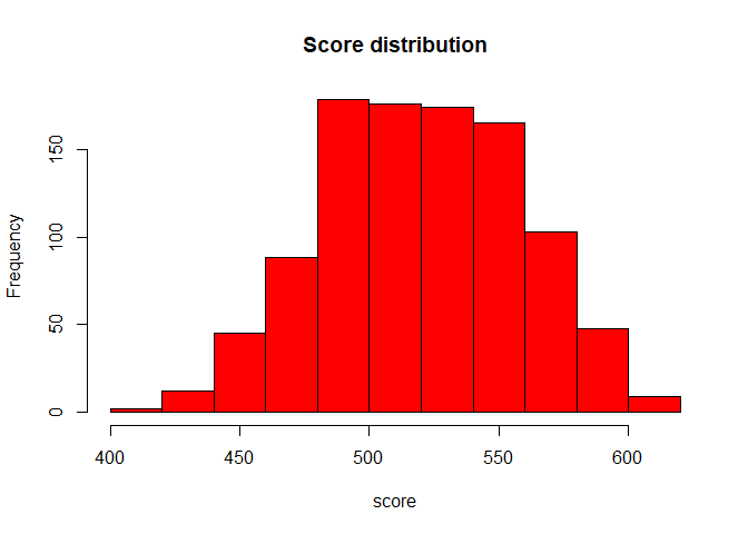
pd.db$score <- round(scaled.score(probs = pd.db$probs, score = 600, odd = 50/1, pdo = 20), 0)
hist(pd.db$score, col = "red", main = "Score distribution", xlab = "score")
#create ratings based on binning algorithm
pd.db$rating <- monobin::sts.bin(x = pd.db$score, y = pd.db$Creditability, y.type = "bina")[[2]]
#summarise rating scale
rs <- pd.db %>%
    group_by(rating) %>%
    summarise(no = n(),
            nb = sum(Creditability),
            ng = sum(1 - Creditability)) %>%
    mutate(dr = nb / no)
rs
## # A tibble: 6 x 5
## rating no nb ng dr
## <chr> <int> <dbl> <dbl> <dbl>
## 1 01 (-Inf,473) 99 75 24 0.758
## 2 02 [473,482) 72 46 26 0.639
## 3 03 [482,506) 196 83 113 0.423
## 4 04 [506,515) 100 30 70 0.3
## 5 05 [515,547) 267 52 215 0.195
## 6 06 [547,Inf) 266 14 252 0.0526Often default rate from the modeling data set differs from the
so-called portfolio central tendency (in practice known as long-run
average). Without going deeper into reasons and direction of this
difference we will assume that central tendency for this case study is
27% and re-calibrate our rating scale. In order to do so, we will use
rs.calibration function from PDtoolkit
package. For details on calibration options check its help page
?rs.calibration.
rs$pd <- rs.calibration(rs = rs,
                dr = "dr",
                w = "no",
                ct = 0.27,
                min.pd = 0.05,
                method = "log.odds.ab")[[1]]
rs
## # A tibble: 6 x 6
## rating no nb ng dr pd
## <chr> <int> <dbl> <dbl> <dbl> <dbl>
## 1 01 (-Inf,473) 99 75 24 0.758 0.740
## 2 02 [473,482) 72 46 26 0.639 0.607
## 3 03 [482,506) 196 83 113 0.423 0.375
## 4 04 [506,515) 100 30 70 0.3 0.252
## 5 05 [515,547) 267 52 215 0.195 0.154
## 6 06 [547,Inf) 266 14 252 0.0526 0.05#check if calibration is performed as expected
sum(rs$pd * rs$no) / sum(rs$no)## [1] 0.27#plot main rating scale characteristics
bp <- barplot(rs$no, names.arg = rs$rating, cex.names = 0.8, las = 2, ylim = c(0, max(rs$no) * 1.2),
main = "Number of observations and default rate per rating")
xlim <- c(floor(min(bp)), ceiling(max(bp)))
par(new = TRUE)
plot(bp, rs$pd, type = "l", col = "red", xaxt = "n", yaxt = "n",
xlab = "", ylab = "", xlim = xlim, ylim = c(0, 1))
text(x = bp, y = rs$pd, label = paste0(round(100 * rs$pd, 2), "%"), col = "red",
cex = 0.6, pos = 3)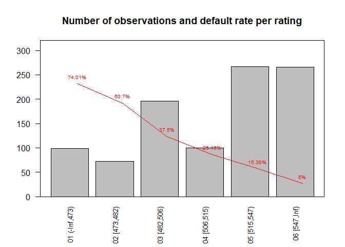
#bring PDs to the modeling data set and calculate AUC
pd.db <- merge(pd.db, rs[, c("rating", "pd")], by = "rating", all.x = TRUE)
auc.model(predictions = pd.db$pd, observed = pd.db$Creditability)
## [1] 0.79465After finalization of PD model development, analysts have to perform
regular validation of the model performance. Model validation is
performed at least on yearly basis on so-called application portfolio.
PDtoolkit has set of functions that are useful for model
validation and next steps present its usage. Before implementation of
any of the validation tests, let’s simulate application portfolio.
set.seed(112233)
app.port <- pd.db[sample(1:nrow(pd.db), 500, replace = FALSE), ]
Now, let’s perform heterogeneity test of the rating scale in order to check if the model still discriminates well between rating grades. This validation procedure applies test of two proportions on adjacent rating grades and check if there is statistical significant difference between observed default rates. It is always one-tail test, but direction depends on direction of default rate per rating (increasing or decreasing).
heterogeneity(app.port = app.port,
          def.ind = "Creditability",
          rating = "rating",
          alpha = 0.05)
## rating no nb dr p.val alpha
## 1 01 (-Inf,473) 47 36 0.76595745 NA 0.05
## 2 02 [473,482) 35 21 0.60000000 0.05319294 0.05
## 3 03 [482,506) 93 37 0.39784946 0.02028868 0.05
## 4 04 [506,515) 53 15 0.28301887 0.08176299 0.05
## 5 05 [515,547) 131 22 0.16793893 0.03889198 0.05
## 6 06 [547,Inf) 141 11 0.07801418 0.01161535 0.05
## res
## 1 <NA>
## 2 H0: DR(02 [473,482)) >= DR(01 (-Inf,473))
## 3 H1: DR(03 [482,506)) < DR(02 [473,482))
## 4 H0: DR(04 [506,515)) >= DR(03 [482,506))
## 5 H1: DR(05 [515,547)) < DR(04 [506,515))
## 6 H1: DR(06 [547,Inf)) < DR(05 [515,547))Based on the results we can see that there are two pairs of rating grades where we cannot conclude that observed default rate in the second rating grade is less than observed default rate in the previous rating grade. These two pairs are:
Usually in practice the further investigation is performed in order
to better understand source of poor discrimination between these two
rating pairs. Due to the fact that application portfolio in this
example does not have enough observations to perform homogeneity test,
the help page of the ?homogeneity function contains
examples, details and design behind the implemented test. Closely
related validation procedure to heterogeneity and homogeneity is
validation of discriminatory power of the PD model. Namely, analysts
usually have to validate and make sure that discriminatory power of the
PD model in use did not deteriorate significantly from the moment of its
development. In order to test the discriminatory power of the PD model
in use, we will apply dp.testing function for the
PDtoolkit package.
#calculate again the AUC for the development sample
auc.dev <- auc.model(predictions = pd.db$pd, observed = pd.db$Creditability)
auc.dev
## [1] 0.79465#test possible AUC deterioration on the application portfolio
dp.testing(app.port = app.port,
def.ind = "Creditability",
pdc = "pd",
auc.test = auc.dev,
alternative = "less",
alpha = 0.05)## auc auc.test estimate auc.se test.stat p.val alpha res
## 1 0.7821032 0.79465 -0.01254677 0.0247617 -0.5067005 0.3061825 0.05 H0: AUC >= AUC testSo, from the validation results, we can conclude that slight decrease
of AUC in application portfolio in comparison to development sample
cannot be considered as statistically significant for significance level
of 5%. Beside the discriminatory power, analysts are also interested in
testing the predictive ability of PD model in use. The
PDtoolkit package has pp.testing function that
can be used for this purpose. Four tests are supported in this
validation function: three of them refer to testing on the rating grade
level (binomial, Jeffreys, z-score), while one refers to the complete
rating scale (Hosmer-Lemeshow test). The null hypothesis for the
binomial, Jeffreys, and z-score test is that the calibrated PDs are not
underestimated, i.e. they are not significantly lower than the observed
default rate, while for the Hosmer-Lemeshow test is that the calibrated
PD is the true one.
#summarise application portfolio to rating grade level
rs.ap <- app.port %>%
       group_by(rating) %>%
       summarise(no = n(),
             nb = sum(Creditability),
             ng = sum(1 - Creditability)) %>%
       mutate(dr = nb / no)
#bring calibrated pd as a based for predictive power testing
rs.ap <- merge(rs[, c("rating", "pd")], rs.ap, by = "rating", all.x = TRUE)
rs.ap
## rating pd no nb ng dr
## 1 01 (-Inf,473) 0.7400826 47 36 11 0.76595745
## 2 02 [473,482) 0.6069830 35 21 14 0.60000000
## 3 03 [482,506) 0.3750350 93 37 56 0.39784946
## 4 04 [506,515) 0.2516151 53 15 38 0.28301887
## 5 05 [515,547) 0.1537853 131 22 109 0.16793893
## 6 06 [547,Inf) 0.0500000 141 11 130 0.07801418#perform predictive power testing
pp.testing(rating.label = rs.ap$rating,
pdc = rs.ap$pd,
no = rs.ap$no,
nb = rs.ap$nb,
alpha = 0.05)## rating no nb odr pdc alpha binomial binomial.res jeffreys
## 1 01 (-Inf,473) 47 36 0.76595745 0.7400826 0.05 0.4159984 H0: ODR <= PDC 0.35159815
## 2 02 [473,482) 35 21 0.60000000 0.6069830 0.05 0.6059111 H0: ODR <= PDC 0.53854844
## 3 03 [482,506) 93 37 0.39784946 0.3750350 0.05 0.3613128 H0: ODR <= PDC 0.32231637
## 4 04 [506,515) 53 15 0.28301887 0.2516151 0.05 0.3479606 H0: ODR <= PDC 0.29276184
## 5 05 [515,547) 131 22 0.16793893 0.1537853 0.05 0.3621511 H0: ODR <= PDC 0.31876653
## 6 06 [547,Inf) 141 11 0.07801418 0.0500000 0.05 0.0966087 H0: ODR <= PDC 0.07085215
## jeffreys.res zscore zscore.res hosmer.lemeshow hosmer.lemeshow.res
## 1 H0: ODR <= PDC 0.34293973 H0: ODR <= PDC 0.7851538 H0: PDC is TRUE
## 2 H0: ODR <= PDC 0.53370338 H0: ODR <= PDC 0.7851538 H0: PDC is TRUE
## 3 H0: ODR <= PDC 0.32475205 H0: ODR <= PDC 0.7851538 H0: PDC is TRUE
## 4 H0: ODR <= PDC 0.29914802 H0: ODR <= PDC 0.7851538 H0: PDC is TRUE
## 5 H0: ODR <= PDC 0.32669329 H0: ODR <= PDC 0.7851538 H0: PDC is TRUE
## 6 H0: ODR <= PDC 0.06346722 H0: ODR <= PDC 0.7851538 H0: PDC is TRUEAs we can see from the results, all three tests rejected the
hypothesis of underestimation of the calibrated PD in comparison to the
observed default rate and Hosmer-Lemeshow test that PD is not the true
one. Sometimes the tests that serve the same purpose can produce
opposite results (lead to opposite conclusions) leaving analysts in
dilemma about overall conclusion. For that purpose we developed the
function power which implements simple framework of power
analysis of the statistical tests. More concretely, this function
calculates the power of the four tests used for predictive ability
testing. Assumption of the power analysis is that observed default rate
is the real default rate, so the ultimate goal of this analysis is to
quantify ability of each statistical test to detect the difference
between the calibrated and real default rate.
power(rating.label = rs.ap$rating,
    pdc = rs.ap$pd,
    no = rs.ap$no,
    nb = rs.ap$nb,
    alpha = 0.05,
    sim.num = 1000,
    seed = 2211)
## $interval.estimator
## rating no nb odr pdc binomial jeffreys zscore
## 1 01 (-Inf,473) 47 36 0.76595745 0.7400826 0.051 0.120 0.120
## 2 02 [473,482) 35 21 0.60000000 0.6069830 0.016 0.053 0.053
## 3 03 [482,506) 93 37 0.39784946 0.3750350 0.087 0.125 0.125
## 4 04 [506,515) 53 15 0.28301887 0.2516151 0.088 0.142 0.142
## 5 05 [515,547) 131 22 0.16793893 0.1537853 0.095 0.095 0.141
## 6 06 [547,Inf) 141 11 0.07801418 0.0500000 0.287 0.391 0.391
##
## $hosmer.lemeshow
## rating
## 1 01 (-Inf,473) + 02 [473,482) + 03 [482,506) + 04 [506,515) + 05 [515,547) + 06 [547,Inf)
## hosmer.lemeshow
## 1 0.268For this application portfolio characteristic we can conclude that in
average higher power of detecting the real underestimation of calibrated
PD have Jeffreys and z-score in comparison to the binomial test. Since
the Hosmer-Lemeshow test is the only test applied to the complete rating
scale, there is no other test to be compared with. For
additional package features that are implemented but not presented in
the above examples, please, check
help(package = "PDtoolkit").