NobBS: Nowcasting by Bayesian Smoothing

NobBS is Bayesian approach to estimate the number of occurred-but-not-yet-reported cases from incomplete, time-stamped reporting data for disease outbreaks. NobBS learns the reporting delay distribution and the time evolution of the epidemic curve to produce smoothed nowcasts in both stable and time-varying case reporting settings. For details, see the publication by McGough et al. 2020.

Installation

You can install the released version of NobBS from CRAN with:

install.packages("NobBS")

The development version of NobBS can be installed with:

library(devtools) 
install_github("sarahhbellum/NobBS")

NobBS requires that JAGS (Just Another Gibbs Sampler) is downloaded to the system or computer on which NobBS will run. Download JAGS here: https://mcmc-jags.sourceforge.io/.

Usage

NobBS accepts a line list of case onset and case reporting dates as the input data, and users are required to specify:

data: A data frame containing the line list data
now: The date at which the nowcast is to be performed (of class Date, e.g. as.Date())
units: The temporal unit of reporting, either “1 day” or “1 week”
onset_date: A string indicating the Date column containing the date of case onset
report_date: A string indicating the Date column containing the date of case report

For example, in the data denguedat, cases are reported on a weekly basis:

library(NobBS)
data(denguedat)
head(denguedat)
#>   onset_week report_week
#> 1 1990-01-01  1990-01-01
#> 2 1990-01-01  1990-01-01
#> 3 1990-01-01  1990-01-01
#> 4 1990-01-01  1990-01-08
#> 5 1990-01-01  1990-01-08
#> 6 1990-01-01  1990-01-15

For this dengue report line list, the user would specify units=“1 week”, onset_date=“onset_week”, and report_date=“report_week” to produce a nowcast for the Date now of choice.

The user may optionally specify arguments such as:

moving_window: The numeric size of the moving window used in the estimation of cases. The default option is NULL, i.e. no moving window, to consider all possible historical dates
max_D: The numeric maximum delay D to consider in the estimation of cases, in the same units as units. For example, if cases are known to be 100% reported within the first 10 weeks, then it would be reasonable to set max_D = 9 weeks. Even if there are longer delays in the data, the delay probability for long delays would be modeled as Pr(Delay ≥ 9weeks). Note that it is not possible to set the maximum delay to be longer than what is possible to observe in the data (e.g. one cannot set max_D=15 in a 12-week time series). By default, max_D is set equal to either:
- the length of the reporting time series minus 1, e.g. if 27 weeks of reporting data are provided, max_D=26.
- the length of moving_window-1, if moving_window is specified.
cutoff_D: A logical argument (default: TRUE) indicating whether to ignore delays larger than max_D. For example, for a moving_window of 27 weeks and a max_D of 10 weeks, cutoff_D = TRUE would indicate that cases reported with an 11+ week delay would be ignored. Conversely, setting cutoff_D=FALSE would model delays longer than 10 weeks within the moving window as Pr(27weeks > Delay ≥ 10weeks).
proportion_reported: A decimal between (0, 1] indicating the expected proportion reported. Default=1, meaning that 100% of cases are expected to be eventually reported. However, this may not be the case in all disease settings; for example, if the disease contributes to a number of asymptomatic cases that will not lead to detection by the health system, or if severe under-reporting is expected during a large outbreak. In these cases, the nowcast estimates will be inflated by 1/proportion_reported.

Bayesian parameters

The user may specify whether underlying cases occur as part of a Poisson or a Negative Binomial process (Default: Poisson), and may specify the priors on the log-linear model as described in McGough et al. 2020, where default values are set to be weakly informative. In addition, arguments governing the JAGS model MCMC sampling may be specified: number of chains (nChains, default=1), number of samples (nSamp, default=10,000), number of iterations discarded as burn-in (nBurnin, default=1000), number of thinned iterations (nThin, default=1), and adaptation period (nAdapt, default=1000). The percentile of the prediction interval may be specified with conf (default = 0.95 for a 95% prediction interval).

For recommendations on priors and moving windows, see the Materials and Methods sub-section in McGough et al. 2020 entitled “NobBS R package implementation and recommendations.”

Model output

Altogether, a simple model may be run by specifying only the required arguments:

NobBS(denguedat, as.Date("1990-10-01"),units="1 week",onset_date="onset_week",report_date="report_week"). The user should save the output to an R object because many levels of information are stored in the output.

test_nowcast <- NobBS(data=denguedat, now=as.Date("1990-10-01"),
                      units="1 week",onset_date="onset_week",report_date="report_week")
#> [1] "Computing a nowcast for  1990-10-01"
#> Compiling model graph
#>    Resolving undeclared variables
#>    Allocating nodes
#> Graph information:
#>    Observed stochastic nodes: 820
#>    Unobserved stochastic nodes: 822
#>    Total graph size: 5090
#> 
#> Initializing model

NobBS returns the list test_nowcast, which contains the following elements:

estimates, accessed via test_nowcast$estimates. This is a 5-column data frame containing case estimates for each date in the historical time series through now, with corresponding date of case onset, lower and upper bounds of the prediction interval, and the number of cases for that onset date reported up to now.
estimates.inflated, accessed via test_nowcast$estimates.inflated. This is a 5-column data frame containing case estimates for each date in the historical time series through now, inflated by the proportion_reported, with corresponding date of case onset, lower and upper bounds of the prediction interval, and the number of cases for that onset date reported up to now.
nowcast.post.samples, accessed via test_nowcasts$nowcast.post.samples. This is a vector of 10,000 samples from the posterior predictive distribution of the nowcast itself.
params.post, accessed via test_nowcast$params.post. This is a data frame containing 10,000 posterior samples for all parameters of the Bayesian model, including α_t = now, {log(β_d),…,log(β_*max**D) }, λt, d, and τα*². This data frame can get increasingly large as the length of the time series of available data increases, so the user can control which parameter’s posterior samples are outputted in specs$param_names (Default: all). See NobBS help file for details of specs.

tail(test_nowcast$estimates)
#>    estimate lower upper onset_date n.reported
#> 35       48    44    53 1990-08-27         44
#> 36       59    55    65 1990-09-03         54
#> 37       45    40    52 1990-09-10         38
#> 38       90    81   101 1990-09-17         71
#> 39       80    65    99 1990-09-24         40
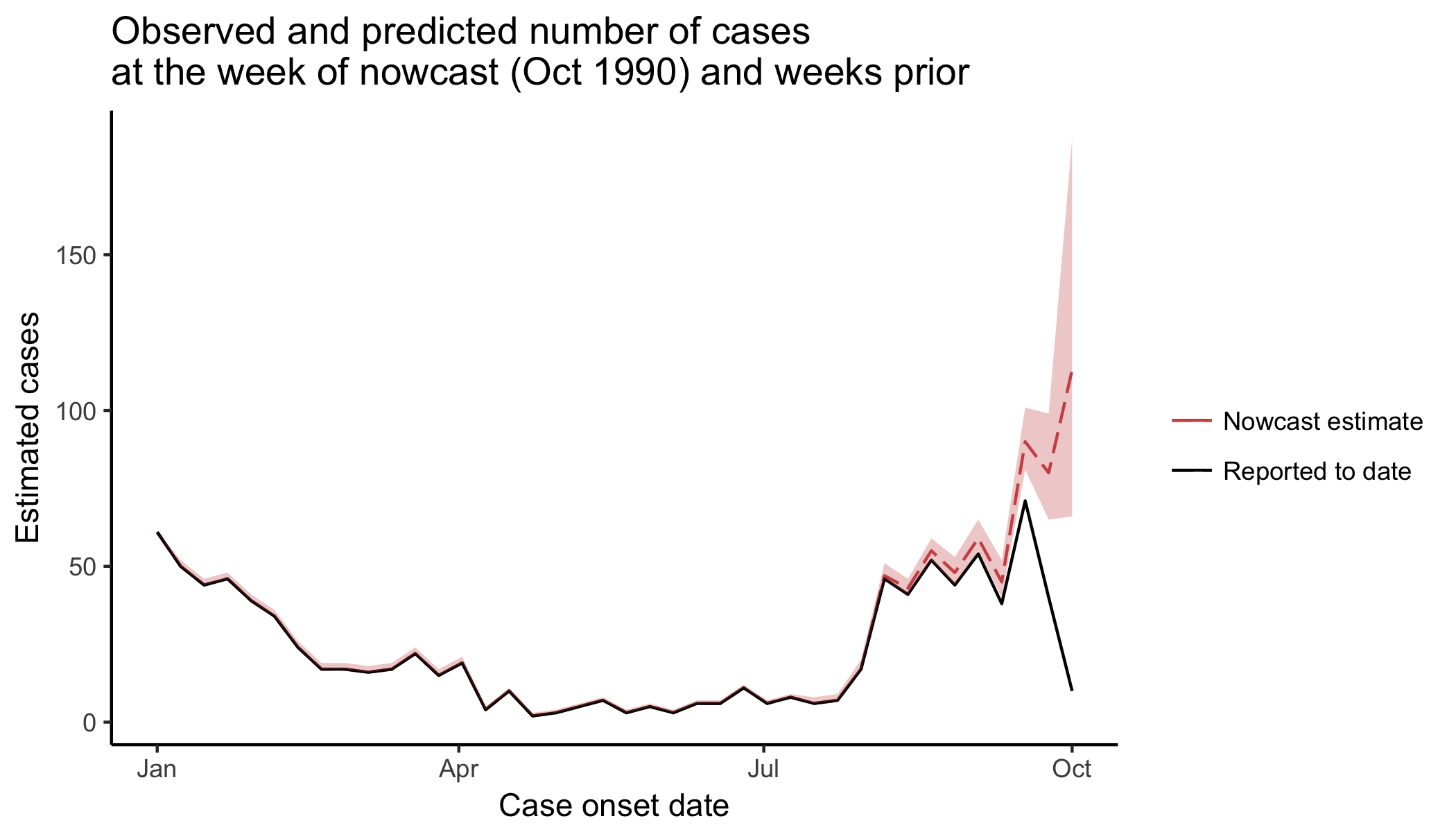
#> 40      113    66   187 1990-10-01         10

Plotting results

The NobBS output can be used in a variety of ways- for example, to inspect the posterior distribution of the nowcast estimate or to plot the nowcast and “hindcasts” (estimates produced for weeks in the past).

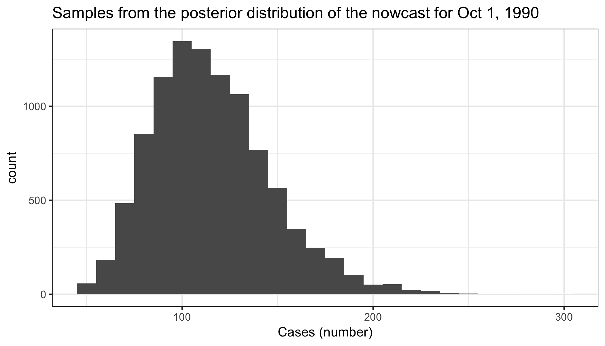
Inspecting the posterior distribution of key parameters

Posterior of the nowcast:

library(ggplot2)
nowcast_posterior <- data.frame(sample_estimate=test_nowcast$nowcast.post.samps)
ggplot(nowcast_posterior, aes(sample_estimate)) + 
  geom_histogram(binwidth=10) + 
  theme_bw() + 
  xlab("Cases (number)") +
  ggtitle("Samples from the posterior distribution of the nowcast for Oct 1, 1990")

Posterior of β_d = 0 (the estimated probability of a case being reported with no delay):

library(ggplot2)
library(dplyr)
beta_0 <- data.frame(prob=exp(test_nowcast$params.post$`Beta 0`))
ggplot(beta_0, aes(prob)) + 
  geom_histogram() + 
  theme_bw() + 
  xlab("Probability of delay=0") +
  ggtitle("Posterior distribution of the probability of delay d=0,
         estimated over the period Jan 1, 1990 to Oct 1, 1990")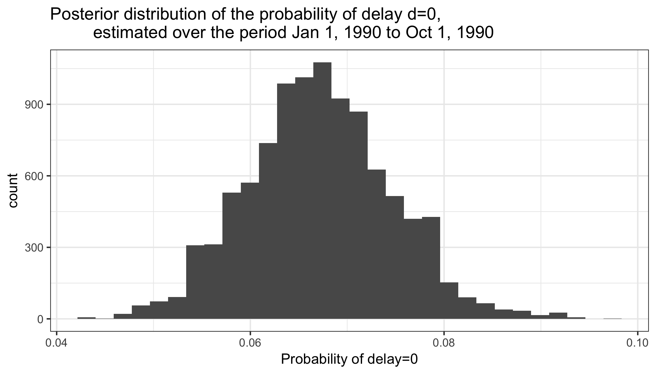

Plotting the sequence of nowcast and hindcasts

nowcasts <- data.frame(test_nowcast$estimates)

ggplot(nowcasts) + geom_line(aes(onset_date,estimate,col="Nowcast estimate"),linetype="longdash") +
  geom_line(aes(onset_date,n.reported,col="Reported to date"),linetype="solid") +
  scale_colour_manual(name="",values=c("indianred3","black"))+
  theme_classic()+
  geom_ribbon(fill="indianred3",aes(x = onset_date,ymin=nowcasts$lower, 
                             ymax=nowcasts$upper),alpha=0.3)+
  xlab("Case onset date") + ylab("Estimated cases") +
  ggtitle("Observed and predicted number of cases \nat the week of nowcast (Oct 1990) and weeks prior")