![]()
![]()
![]()
This package provides functions that make it easy to get plottable predictions from multinomial logit models. The predictions are based on simulated draws of regression estimates from their respective sampling distribution.
At first I will present the theoretical and statistical background, before using sample data to demonstrate the functions of the package.
For the statistical and theoretical background of the multinomial logit regression please refer to the vignette or sources like these lecture notes by Germán Rodríguez.
Due to the inconvenience of integrating math equations in the README file, this is not the place to write comprehensively about it.
These are the important characteristics of the model:
This package helps to interpret the model in meaningful ways.
The package can be both installed from CRAN or the github repository:
# Uncomment if necessary:

# install.packages("MNLpred")
# devtools::install_github("ManuelNeumann/MNLpred")As we have seen above, the multinomial logit can be used to get an insight into the probabilities to choose one option out of a set of alternatives. We have also seen that we need a baseline category to identify the model. This is mathematically necessary, but does not come in handy for purposes of interpretation.
It is far more helpful and easier to understand to come up with predicted probabilities and first differences for values of interest (see e.g., King, Tomz, and Wittenberg 2000 for approaches in social sciences). Based on simulations, this package helps to easily predict probabilities and their uncertainty in forms of confidence intervals for each choice category over a specified scenario. The functions use the observed values to compute the predicted probabilities, as is recommended by Hanmer and Ozan Kalkan (2013).
The procedure follows the following steps:
The presented functions follow these steps. Additionally, they use the so called observed value approach. This means that the “scenario” uses all observed values that informed the model. Therefore the function takes these more detailed steps:
For first differences, the simulated predictions are subtracted from each other.
To showcase these steps, I present a reproducible example of how the functions can be used.
The example uses data from the German Longitudinal Election Study (GLES, Roßteutscher et al. (2019)).
The contains 1,000 respondents characteristics and their vote choice.
For this task, we need the following packages:
# Required packages
library(magrittr) # for pipes
library(nnet) # for the multinom()-function
library(MASS) # for the multivariate normal distribution

# The package
library(MNLpred)

# Plotting the predicted probabilities:
library(ggplot2)
library(scales)
Now we load the data:
# The data:
data("gles")
The next step is to compute the actual model. The function of the
MNLpred package is based on models that were estimated with
the multinom()-function of the nnet package.
The multinom() function is convenient because it does not
need transformed datasets. The syntax is very easy and resembles the
ordinary regression functions. Important is that the Hessian matrix is
returned with Hess = TRUE. The matrix is needed to simulate
the sampling distribution.
As we have seen above, we need a baseline or reference category for
the model to work. Therefore, be aware what your baseline category is.
If you use a dependent variable that is of type character,
the categories will be ordered in alphabetical order. If you have a
factorat hand, you can define your baseline category, for
example with the relevel()function.
Now, let’s estimate the model:
# Multinomial logit model:
mod1 <- multinom(vote ~ egoposition_immigration +
                   political_interest +
                   income + gender + ostwest,
                 data = gles,
                 Hess = TRUE)
#> # weights:  42 (30 variable)
#> initial  value 1791.759469
#> iter  10 value 1644.501289
#> iter  20 value 1553.803188
#> iter  30 value 1538.792079
#> final  value 1537.906674
#> converged
The results show the coefficients and standard errors. As we can see,
there are five sets of coefficients. They describe the relationship
between the reference category (AfD) and the vote choices
for the parties CDU/CSU, FDP,
Gruene, LINKE, and SPD.
summary(mod1)
#> Call:
#> multinom(formula = vote ~ egoposition_immigration + political_interest +
#>     income + gender + ostwest, data = gles, Hess = TRUE)
#>
#> Coefficients:
#>         (Intercept) egoposition_immigration political_interest      income
#> CDU/CSU    3.101201              -0.4419104        -0.29177070  0.33114348
#> FDP        2.070618              -0.4106626        -0.19044703  0.18496691
#> Gruene     3.232074              -0.8482213        -0.03023454  0.24330589
#> LINKE      4.990008              -0.7477359        -0.04503371 -0.24206850
#> SPD        3.799394              -0.6425427        -0.03514426  0.08211066
#>           gender     ostwest
#> CDU/CSU 1.296949  0.79760035
#> FDP     1.252112  1.01378955
#> Gruene  1.831714  0.76299897
#> LINKE   1.368591 -0.02428322
#> SPD     1.497019  0.74026388
#>
#> Std. Errors:
#>         (Intercept) egoposition_immigration political_interest    income
#> CDU/CSU   0.8568928              0.06504100          0.1694270 0.1872533
#> FDP       0.9508589              0.07083385          0.1882974 0.2063590
#> Gruene    0.9854950              0.07887427          0.1969704 0.2149368
#> LINKE     0.9505656              0.07755359          0.1962954 0.2058036
#> SPD       0.8880256              0.06912678          0.1779570 0.1924002
#>            gender   ostwest
#> CDU/CSU 0.3530225 0.3120178
#> FDP     0.3794295 0.3615071
#> Gruene  0.3875116 0.3671397
#> LINKE   0.3885663 0.3493941
#> SPD     0.3625652 0.3269007
#>
#> Residual Deviance: 3075.813
#> AIC: 3135.813
A first rough review of the coefficients shows that a more restrictive ego-position toward immigration leads to a lower probability of the voters to choose any other party than the AfD. It is hard to evaluate whether the effect is statistically significant and how the probabilities for each choice look like. For this it is helpful to predict the probabilities for certain scenarios and plot the means and confidence intervals for visual analysis.
Let’s say we are interested in the relationship between the ego-position toward immigration and the probability to choose any of the parties. It would be helpful to plot the predicted probabilities for the span of the positions.
summary(gles$egoposition_immigration)
#>    Min. 1st Qu.  Median    Mean 3rd Qu.    Max.
#>   0.000   3.000   4.000   4.361   6.000  10.000
As we can see, the ego positions were recorded on a scale from 0 to
10. Higher numbers represent more restrictive positions. We pick this
score as the x-variable (x) and use the
mnl_pred_ova() function to get predicted probabilities for
each position in this range.
The function needs a multinomial logit model (model),
data (data), the variable of interest x, the
steps for which the probabilities should be predicted (by).
Additionally, a seed can be defined for replication
purposes, the numbers of simulations can be defined (nsim),
and the confidence intervals (probs).
If we want to hold another variable stable, we can specify so with
zand z_value. See also the
mnl_fd_ova() function below.
pred1 <- mnl_pred_ova(model = mod1,
                      data = gles,
                      x = "egoposition_immigration",
                      by = 1,
                      seed = 68159,
                      nsim = 100, # faster
                      probs = c(0.025, 0.975)) # default
#> Multiplying values with simulated estimates:
#> ================================================================================
#> Applying link function:
#> ================================================================================
#> Done!
The function returns a list with several elements. Most importantly,
it returns a plotdata data set:
pred1$plotdata %>% head()
#>   egoposition_immigration vote        mean       lower       upper
#> 1                       0  AfD 0.002419192 0.001025942 0.004913258
#> 2                       1  AfD 0.004625108 0.002172854 0.008685788
#> 3                       2  AfD 0.008653845 0.004472502 0.014698651
#> 4                       3  AfD 0.015796304 0.008923480 0.025148142
#> 5                       4  AfD 0.028022769 0.017756232 0.040861062
#> 6                       5  AfD 0.048081830 0.033241425 0.063794110
As we can see, it includes the range of the x variable, a mean, a
lower, and an upper bound of the confidence interval. Concerning the
choice category, the data is in a long format. This makes it easy to
plot it with the ggplot syntax. The choice category can now
easily be used to differentiate the lines in the plot by using
linetype = vote in the aes(). Another option
is to use facet_wrap() or facet_grid() to
differentiate the predictions:
ggplot(data = pred1$plotdata, aes(x = egoposition_immigration,
                                  y = mean,
                                  ymin = lower, ymax = upper)) +
  geom_ribbon(alpha = 0.1) + # Confidence intervals
  geom_line() + # Mean
  facet_wrap(.~ vote, scales = "free_y", ncol = 2) +
  scale_y_continuous(labels = percent_format(accuracy = 1)) + # % labels
  scale_x_continuous(breaks = c(0:10),
                     minor_breaks = FALSE) +
  theme_bw() +
  labs(y = "Predicted probabilities",
       x = "Ego-position toward immigration") # Always label your axes ;)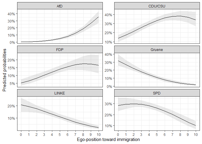
If we want first differences between two scenarios, we can use the
function mnl_fd2_ova(). The function takes similar
arguments as the function above, but now the values for the scenarios of
interest have to be supplied. Imagine we want to know what difference it
makes to position oneself on the most tolerant or most restrictive end
of the egoposition_immigration scale. This can be done as
follows:
fdif1 <- mnl_fd2_ova(model = mod1,
                     data = gles,
                     x = "egoposition_immigration",
                     value1 = min(gles$egoposition_immigration),
                     value2 = max(gles$egoposition_immigration),
                     seed = 68159,
                     nsim = 100)
#> Multiplying values with simulated estimates:
#> ================================================================================
#> Applying link function:
#> ================================================================================
#> Done!
The first differences can then be depicted in a graph.
ggplot(fdif1$plotdata_fd, aes(x = categories,
                              y = mean,
                              ymin = lower, ymax = upper)) +
  geom_pointrange() +
  geom_hline(yintercept = 0) +
  scale_y_continuous(labels = percent_format()) +
  theme_bw() +
  labs(y = "Predicted probabilities",
       x = "Party vote")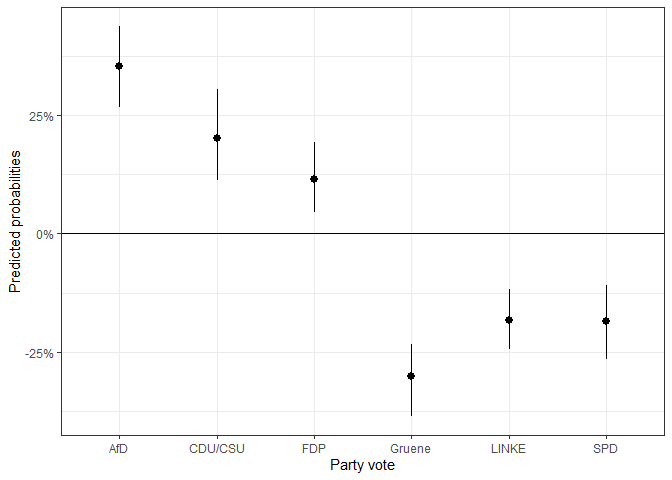
We are often not only interested in the static difference, but the
difference across a span of values, given a difference in a second
variable. This is especially helpful when we look at dummy variables.
For example, we could be interested in the effect of gender
on the vote decision over the different ego-positions. With the
mnl_fd_ova() function, we can predict the probabilities for
two scenarios and subtract them. The function returns the differences
and the confidence intervals of the differences. The different scenarios
can be held stable with z and the z_values.
z_values takes a vector of two numeric values. These values
are held stable for the variable that is named in z.
fdif2 <- mnl_fd_ova(model = mod1,
                    data = gles,
                    x = "egoposition_immigration",
                    by = 1,
                    z = "gender",
                    z_values = c(0,1),
                    seed = 68159,
                    nsim = 100)
#> First scenario:
#> Multiplying values with simulated estimates:
#> ================================================================================
#> Applying link function:
#> ================================================================================
#> Done!
#>
#> Second scenario:
#> Multiplying values with simulated estimates:
#> ================================================================================
#> Applying link function:
#> ================================================================================
#> Done!
As before, the function returns a list including a data set that can be used to plot the differences.
fdif2$plotdata_fd %>% head()
#>   egoposition_immigration vote         mean        lower        upper
#> 1                       0  AfD -0.002861681 -0.006172786 -0.001206796
#> 2                       1  AfD -0.005396410 -0.010531302 -0.002537904
#> 3                       2  AfD -0.009942124 -0.017921934 -0.005038667
#> 4                       3  AfD -0.017827751 -0.029548569 -0.009657235
#> 5                       4  AfD -0.030957366 -0.046960384 -0.017810853
#> 6                       5  AfD -0.051691516 -0.071903589 -0.031438906
Since the function calls the mnl_pred_ova() function
internally, it also returns the output of the two predictions in the
list element Prediction1 and Prediction2. The
plot data for the predictions is already bound together row wise to
easily plot the predicted probabilities.
ggplot(data = fdif2$plotdata, aes(x = egoposition_immigration,
                                  y = mean,
                                  ymin = lower, ymax = upper,
                                  group = as.factor(gender),
                                  linetype = as.factor(gender))) +
  geom_ribbon(alpha = 0.1) +
  geom_line() +
  facet_wrap(. ~ vote, scales = "free_y", ncol = 2) +
  scale_y_continuous(labels = percent_format(accuracy = 1)) + # % labels
  scale_x_continuous(breaks = c(0:10),
                     minor_breaks = FALSE) +
  scale_linetype_discrete(name = "Gender",
                          breaks = c(0, 1),
                          labels = c("Male", "Female")) +
  theme_bw() +
  labs(y = "Predicted probabilities",
       x = "Ego-position toward immigration") # Always label your axes ;)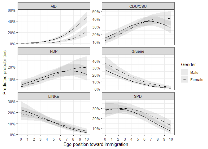
As we can see, the differences between female and
male differ, depending on the party and ego-position. So
let’s take a look at the differences:
ggplot(data = fdif2$plotdata_fd, aes(x = egoposition_immigration,
                                     y = mean,
                                  ymin = lower, ymax = upper)) +
  geom_ribbon(alpha = 0.1) +
  geom_line() +
  geom_hline(yintercept = 0) +
  facet_wrap(. ~ vote, ncol = 3) +
  scale_y_continuous(labels = percent_format(accuracy = 1)) + # % labels
  scale_x_continuous(breaks = c(0:10),
                     minor_breaks = FALSE) +
  theme_bw() +
  labs(y = "Predicted probabilities",
       x = "Ego-position toward immigration") # Always label your axes ;)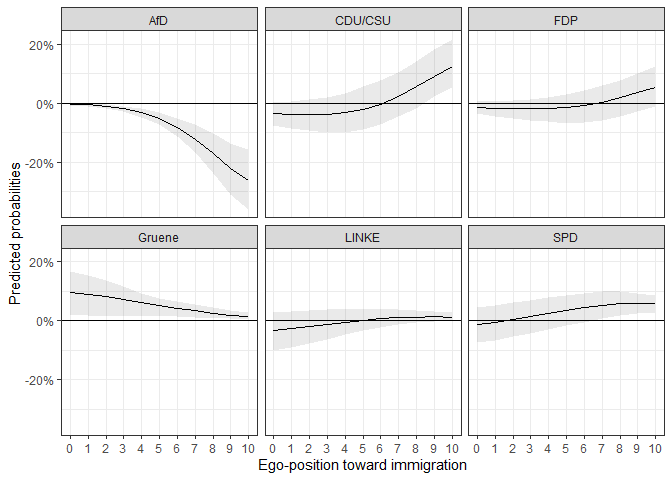
We can see that the differences are for some parties at no point statistically significant from 0.
Multinomial logit models are important to model nominal choices. They
are, however, restricted by being in need of a baseline category.
Additionally, the log-character of the estimates makes it difficult to
interpret them in meaningful ways. Predicting probabilities for all
choices for scenarios, based on the observed data provides much more
insight. The functions of this package provide easy to use functions
that return data that can be used to plot predicted probabilities. The
function uses a model from the multinom() function and uses
the observed value approach and a supplied scenario to predict values
over the range of fitting values. The functions simulate sampling
distributions and therefore provide meaningful confidence intervals.
mnl_pred_ova() can be used to predict probabilities for a
certain scenario. mnl_fd_ova() can be used to predict
probabilities for two scenarios and their first differences.
My code is inspired by the method courses in the Political Science master’s program at the University of Mannheim(cool place, check it out!). The skeleton of the code is based on a tutorial taught by Marcel Neunhoeffer (lecture: “Advanced Quantitative Methods” by Thomas Gschwend).
General DOI (always links to most recent version): 10.5281/zenodo.4525342
DOIs for different versions: