
![]()
The goal of LREP is to estimate the Parameters for the Pareto Distribution and test Pareto vs. Exponential Distributions
You can install the released version of LREP from CRAN with:
install.packages("LREP")And the development version from GitHub with:
# install.packages("devtools")
devtools::install_github("jiqiaingwu/LREP")Our test is a likelihood ratio test of the following hypotheses:
Ho: data comes from an exponential distribution, versus the alternative
H1: data comes from a Pareto distribution.
The approach is to consider the ratio of the maxima of the likelihoods of the observed sample under the Pareto or exponential (in the numerator) and exponential (in the denominator) models. The logarithm (natural) of the likelihood ratio, the L statistic, is:
Where is the observed sample of excesses and
and
are the likelihood functions of the sample
under Pareto and exponential models, respectively.
We use a Pareto distribution with the survival function and exponential distribution with the
survival function
. To compute L, both likelihoods are
maximized first (via maximum likelihood estimates, MLEs, of the
parameters), and then the natural logarithm of their ratio is taken as
the likelihood ratio statistic. Panorska et al. (2007) provide the
necessary theoretical results for the implementation of the numerical
routines necessary for the computation of L. The properties of the test,
proofs and more details on the optimization process appear separately in
Kozubowski et al.(2007)
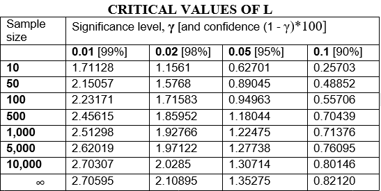
The percentiles of L provide the critical
numbers for our test on the significance level
. The test is one-sided and we reject the
null hypothesis if the computed value of the test statistic exceeds the
critical number. We have computed some common percentiles for the
distribution of L under the null hypothesis for different sample sizes
and for the limiting case. The percentiles for finite sample sizes were
computed via Monte Carlo simulation with 10,000 samples of a given size
from the exponential distribution (Table below).
This is a basic example which shows you how to solve a common problem:
library(LREP)
###example when data is Exponential
####################################
x<-rexp(1000,0.000000000005)
1/mean(x)
#> [1] 4.793131e-12
print(sigmaalphaLREP(x,10^-12))
#>         s.hat     a.hat log.like.ratio
#> [1,] 53706554 0.1300092              0
print(expparetotest(x,0.05))
#>      critical           statistic
#> [1,] "2.44610889355019" "0"
#>      info
#> [1,] "Data is comming from an exponential distribution \n"
##asymptotic p-value
1/2*(1-pchisq(0,df=1))
#> [1] 0.5
x<-rexp(1000,0.1)
1/mean(x)
#> [1] 0.09905136
print(sigmaalphaLREP(x,10^-12))
#>         s.hat    a.hat log.like.ratio
#> [1,] 13081.96 1296.781              0
print(expparetotest(x,0.05))
#>      critical           statistic
#> [1,] "2.44610889355019" "0"
#>      info
#> [1,] "Data is comming from an exponential distribution \n"
##asymptotic p-value
1/2*(1-pchisq(1.596044,df=1))
#> [1] 0.1032324
###example when data is Pareto
####################################
pareto.generation<- function(s,a,n)
{
    u<-runif(n)
    x<-s*((1-u)^(-1/a)-1)
    x
}
x<-pareto.generation(10,7,1000)
print(sigmaalphaLREP(x,10^-12))
#>         s.hat   a.hat log.like.ratio
#> [1,] 8.899638 6.61621       19.66083
print(expparetotest(x,0.05))
#>      critical           statistic
#> [1,] "2.44610889355019" "19.6608276205241"
#>      info
#> [1,] "Data is comming from Pareto distribution \n"
##asymptotic p-value
1/2*(1-pchisq(14.43144,df=1))
#> [1] 7.267762e-05