GPUs are great resources for data analysis, especially in statistics and linear algebra. Unfortunately, very few packages connect R to the GPU, and none of them are transparent enough to run the computations on the GPU without substantial changes to the code. The maintenance of these packages is cumbersome: several of the earlier attempts have been removed from their respective repositories. It would be desirable to have a properly maintained R package that takes advantage of the GPU with minimal changes to the existing code.
We have developed the GPUmatrix package (available on CRAN). GPUmatrix mimics the behavior of the Matrix package and extends R to use the GPU for computations. It includes single(FP32) and double(FP64) precision data types, and provides support for sparse matrices. It is easy to learn, and requires very few code changes to perform the operations on the GPU. GPUmatrix relies on either the Torch or Tensorflow R packages to perform the GPU operations.
We have demonstrated its usefulness for several statistical applications and machine learning applications: non-negative matrix factorization, logistic regression and general linear models. We have also included a comparison of GPU and CPU performance on different matrix operations.
Before starting, please be advised that this R package is designed to have the lowest learning curve for the R user to perform algebraic operations using the GPU. Therefore, this tutorial will mostly cover procedures that will go beyond the operations that the user can already perform with R’s CPU matrices.
GPUmatrix is an R package that utilizes tensors through the torch or tensorflow packages (see Advanced Users section for more information). One or the other must be installed for the use of GPUmatrix. Both packages are hosted in CRAN and have specific installation instructions. In both cases, it is necessary to have an NVIDIA® GPU card with the latest drivers installed in order to use the packages, as well as a version of Python 3. The NVIDIA card must be compatible; please see the list of capable cards here. If there is no compatible graphics card or not graphic card at all, you can still install tensorFlow and torch, but only with the CPU version, which means that GPUmatrix will only be able to run in CPU mode.
install.packages("torch")
library(torch)
install_torch() # In some cases is required.
MUST INSTALL:
The installation of TensorFlow allows the selection to install the
GPU, CPU, or both versions (in Windows the GPU version is no longer
supported). This will depend on the version of TensorFlow that we
install with the install_tensorflow() function. The mode in
which the tensors are created using GPUmatrix, if we choose to use
TensorFlow, will depend on the installation mode. The options to switch
from CPU to GPU are not enabled when using GPUmatrix with TensorFlow for
this precise reason. To install the GPU version, it is not necessary to
specify the version since if it detects that the CUDA dependencies
are met, it will automatically install using the GPU mode. If you
want to install the CPU version, you need to specify it as follows:
install_tensorflow(version="nightly-cpu")
install.packages("tensorflow")
library(tensorflow)
install_tensorflow(version = "nightly-gpu")
MUST INSTALL:
Great news! No additional software required to work on Apple Silicon (either the CPU or the GPU).
Once the dependencies for Torch or TensorFlow are installed, the GPUmatrix package, being a package hosted on CRAN, can be easily installed using:
install.packages("GPUmatrix")Alternatively, it is possible to install the package from GitHub ot get the last version of the package.
devtools::install_github("arubio2/GPUmatrix")The GPUmatrix package is based on S4 objects in R and we have created
a constructor function that acts similarly to the default
matrix() constructor in R for CPU matrices. The constructor
function is gpu.matrix() and accepts the same parameters as
matrix():
library(GPUmatrix)## Torch tensors allowed
## Tensorflow tensors allowed#R matrix initialization
m <- matrix(c(1:20)+40,10,2)
#Show CPU matrix
m## [,1] [,2]
## [1,] 41 51
## [2,] 42 52
## [3,] 43 53
## [4,] 44 54
## [5,] 45 55
## [6,] 46 56
## [7,] 47 57
## [8,] 48 58
## [9,] 49 59
## [10,] 50 60#GPU matrix initialization
Gm <- gpu.matrix(c(1:20)+40,10,2)## Loading required namespace: torch#Show GPU matrix
Gm## GPUmatrix
## torch_tensor
## 41 51
## 42 52
## 43 53
## 44 54
## 45 55
## 46 56
## 47 57
## 48 58
## 49 59
## 50 60
## [ CUDADoubleType{10,2} ]Although the indexing of tensors in both torch and tensorflow is
0-based, the indexing of GPUmatrix objects is 1-based, making it as
close as possible to working with native R matrices and more convenient
for the user. In the previous example, a normal R CPU matrix called
m and its GPU counterpart Gm are created. Just
like regular matrices, the created GPU matrices allow for indexing of
its elements and assignment of values. The concatenation operators
rbind() and cbind() work independently of the
type of matrices that are to be concatenated, resulting in a
gpu.matrix:
Gm[c(2,3),1]## GPUmatrix
## torch_tensor
## 42
## 43
## [ CUDADoubleType{2,1} ]Gm[,2]## GPUmatrix
## torch_tensor
## 51
## 52
## 53
## 54
## 55
## 56
## 57
## 58
## 59
## 60
## [ CUDADoubleType{10,1} ]Gm2 <- cbind(Gm[c(1,2),], Gm[c(6,7),])
Gm2## GPUmatrix
## torch_tensor
## 41 51 46 56
## 42 52 47 57
## [ CUDADoubleType{2,4} ]Gm2[1,3] <- 0
Gm2## GPUmatrix
## torch_tensor
## 41 51 0 56
## 42 52 47 57
## [ CUDADoubleType{2,4} ]It is also possible to initialize the data with NaN values:
Gm3 <- gpu.matrix(nrow = 2,ncol=3)
Gm3[,2]
## GPUmatrix
## torch_tensor
## nan
## nan
## [ CUDADoubleType{2,1} ]Gm3[1,2] <- 1
Gm3## GPUmatrix
## torch_tensor
## nan 1 nan
## nan nan nan
## [ CUDADoubleType{2,3} ]Gm3[1,3] <- 0
Gm3## GPUmatrix
## torch_tensor
## nan 1 0
## nan nan nan
## [ CUDADoubleType{2,3} ]These examples demonstrate that, contrary to standard R, subsetting a gpu.matrix —even when selecting only one column or row— still results in a gpu.matrix. This behavior is analogous to using ‘drop=F’ in standard R. The default standard matrices in R have limitations. The only allowed numeric data types are int and float64. It neither natively allows the creation or handling of sparse matrices. To make up for this lack of functionality, other R packages hosted in CRAN have been created to manage these types.
In the GPUmatrix constructor, we can specify the location of the
matrix, i.e., we can decide to host it on the GPU or in RAM memory to
use it with the CPU. As a package, as its name suggests, oriented
towards algebraic operations in R using the GPU, it will by default be
hosted on the GPU, but it allows the same functionalities using the CPU.
To do this, we use the device attribute of the constructor
and assign it the value “cpu”.
#GPUmatrix initialization with CPU option
Gm <- gpu.matrix(c(1:20)+40,10,2,device="cpu")
#Show CPU matrix from GPUmatrix
Gm
## GPUmatrix
## torch_tensor
## 41 51
## 42 52
## 43 53
## 44 54
## 45 55
## 46 56
## 47 57
## 48 58
## 49 59
## 50 60
## [ CPUDoubleType{10,2} ]The GPUmatrix package also supports Apple Silicon devices, allowing
GPU operations to work seamlessly. By using the
device = "mds" option in most functions, users can leverage
the GPU on Apple Silicon machines out of the box. This ensures optimal
performance on devices equipped with the Apple Silicon Mxx family. In
these GPUs, float64 is not available.
if (installTorch()) {
  # GPUmatrix initialization for Apple Silicon GPU
  Gm <- gpu.matrix(c(1:20)+40,10,2,device="mds")
  # Show Apple Silicon GPU matrix from GPUmatrix
  Gm
}As commented in the introduction and dependency section, GPUmatrix
can be used with both TensorFlow and Torch. By default, the GPU matrix
constructor is initialized with Torch tensors because, in our opinion,
it provides an advantage in terms of installation and usage compared to
TensorFlow. Additionally, it allows the use of GPUmatrix not only with
GPU tensors but also with CPU tensors. To use GPUmatrix with TensorFlow,
simply use the type attribute in the constructor function
and assign it the value “tensorflow” as shown in the
following example:
# library(GPUmatrix)
tensorflowGPUmatrix <- gpu.matrix(c(1:20)+40,10,2, type = "tensorflow") tensorflowGPUmatrixThe default matrices in R have limitations. The numeric data types it allows are int and float64, with float64 being the type used generally in R by default. It also does not natively allow for the creation and handling of sparse matrices. To make up for this lack of functionality, other R packages hosted in CRAN have been created that allow for programming these types of functionality in R. The problem with these packages is that in most cases they are not compatible with each other, meaning we can have a sparse matrix with float64 and a non-sparse matrix with float32, but not a sparse matrix with float32.
GPUmatrix allows for compatibility with sparse matrices and different data types such as float32. For this reason, casting operations between different matrix types from multiple packages to GPUmatrix type have been implemented:
| Matrix class | Package | Data type default | SPARSE | Back cast |
|---|---|---|---|---|
| matrix | base | float64 | FALSE | TRUE |
| data.frame | base | float64 | FALSE | TRUE |
| integer | base | float64 | FALSE | TRUE |
| numeric | base | float64 | FALSE | TRUE |
| dgeMatrix | Matrix | float64 | FALSE | FALSE |
| ddiMatrix | Matrix | float64 | TRUE | FALSE |
| dpoMatrix | Matrix | float64 | FALSE | FALSE |
| dgCMatrix | Matrix | float64 | TRUE | FALSE |
| float32 | float | float32 | FALSE | FALSE |
| torch_tensor | torch | float64 | Depends of tensor type | TRUE |
| tensorflow.tensor | tensorflow | float64 | Depends of tensor type | TRUE |
Table 1. Cast options from other packages. If back cast is TRUE, then it is possible to convert a gpu.matrix to this object and vice versa. If is FALSE, it is possible to convert these objects to gpu.matrix but not vice versa.
There are two functions for casting to create a
gpu.matrix:
as.gpu.matrix() and the
gpu.matrix() constructor itself. Both have
the same input parameters for casting: the object to be cast and extra
parameters for creating a GPUmatrix.
reate ‘Gm’ from ‘m’ matrix R-base:
m <- matrix(c(1:10)+40,5,2)
Gm <- gpu.matrix(m)
Gm
## GPUmatrix
## torch_tensor
## 41 46
## 42 47
## 43 48
## 44 49
## 45 50
## [ CUDADoubleType{5,2} ]Create ‘Gm’ from ‘M’ with Matrix package:
library(Matrix)##
## Attaching package: 'Matrix'
## The following object is masked from 'package:GPUmatrix':
##
## detM <- Matrix(c(1:10)+40,5,2)
Gm <- gpu.matrix(M)
Gm## GPUmatrix
## torch_tensor
## 41 46
## 42 47
## 43 48
## 44 49
## 45 50
## [ CUDADoubleType{5,2} ]Create ‘Gm’ from ‘mfloat32’ with float package:
library(float)
mfloat32 <- fl(m)
Gm <- gpu.matrix(mfloat32)
Gm
## GPUmatrix
## torch_tensor
## 41 46
## 42 47
## 43 48
## 44 49
## 45 50
## [ CUDAFloatType{5,2} ]Interestingly, GPUmatrix returns a float32 data type matrix if the input is a float matrix.
It is also possible to a gpu.matrix create ‘Gms’ type sparse from ‘Ms’ type sparse dgCMatrix, dgeMatrix, ddiMatrix or dpoMatrix with Matrix package:
Ms <- Matrix(sample(0:1, 10, replace = TRUE), nrow=5, ncol=2, sparse=TRUE)
Ms
## 5 x 2 sparse Matrix of class "dgCMatrix"
##
## [1,] 1 .
## [2,] 1 1
## [3,] . 1
## [4,] 1 .
## [5,] . 1Gms <- gpu.matrix(Ms)
Gms## GPUmatrix
## torch_tensor
## [ SparseCUDAFloatType{}
## indices:
## 0 1 1 2 3 4
## 0 0 1 1 0 1
## [ CUDALongType{2,6} ]
## values:
## 1
## 1
## 1
## 1
## 1
## 1
## [ CUDAFloatType{6} ]
## size:
## [5, 2]
## ]The data types allowed by GPUmatrix are: float64,
float32, int, bool or
logical, complex64 and
complex32. We can create a GPU matrix with a specific
data type using the dtype parameter of the
gpu.matrix() constructor function. It is
also possible change the data type of a previously created GPU matrix
using the the data type of a previously created GPU matrix using the
dtype() function. The same applies to GPU
sparse matrices, we can create them from the constructor using the
sparse parameter, which will obtain a
Boolean value of TRUE/FALSE depending on
whether we want the resulting matrix to be sparse or not. We can also
modify the sparsity of an existing GPU matrix with the functions
to_dense(), if we want it to go from
sparse to dense, and to_sparse(), if we
want it to go from dense to sparse.
#Creating a float32 matrix
Gm32 <- gpu.matrix(c(1:20)+40,10,2, dtype = "float32")
Gm32
## GPUmatrix
## torch_tensor
## 41 51
## 42 52
## 43 53
## 44 54
## 45 55
## 46 56
## 47 57
## 48 58
## 49 59
## 50 60
## [ CUDAFloatType{10,2} ]#Creating a non sparse martix with data type float32 from a sparse matrix type float64
Ms <- Matrix(sample(0:1, 20, replace = TRUE), nrow=10, ncol=2, sparse=TRUE)
Gm32 <- gpu.matrix(Ms, dtype = "float32", sparse = F)
Gm32## GPUmatrix
## torch_tensor
## 1 0
## 1 1
## 1 1
## 0 0
## 0 0
## 1 0
## 0 1
## 1 0
## 0 0
## 0 0
## [ CUDAFloatType{10,2} ]#Convert Gm32 in sparse matrix Gms32
Gms32 <- to_sparse(Gm32)
Gms32## GPUmatrix
## torch_tensor
## [ SparseCUDAFloatType{}
## indices:
## 0 1 1 2 2 5 6 7
## 0 0 1 0 1 0 1 0
## [ CUDALongType{2,8} ]
## values:
## 1
## 1
## 1
## 1
## 1
## 1
## 1
## 1
## [ CUDAFloatType{8} ]
## size:
## [10, 2]
## ]##Convert data type Gms32 in float64
Gms64 <- Gms32
dtype(Gms64) <- "float64"
Gms64## GPUmatrix
## torch_tensor
## [ SparseCUDADoubleType{}
## indices:
## 0 1 1 2 2 5 6 7
## 0 0 1 0 1 0 1 0
## [ CUDALongType{2,8} ]
## values:
## 1
## 1
## 1
## 1
## 1
## 1
## 1
## 1
## [ CUDADoubleType{8} ]
## size:
## [10, 2]
## ]GPUmatrix supports all basic arithmetic operators in R:
+, -, *, ^,
/, %*% and %%. Its usage is the
same as for basic R matrices, and it allows compatibility with other
matrix objects from the packages mentioned above.
(Gm + Gm) == (m + m)## [,1] [,2]
## [1,] TRUE TRUE
## [2,] TRUE TRUE
## [3,] TRUE TRUE
## [4,] TRUE TRUE
## [5,] TRUE TRUE(Gm + M) == (mfloat32 + Gm)## [,1] [,2]
## [1,] TRUE TRUE
## [2,] TRUE TRUE
## [3,] TRUE TRUE
## [4,] TRUE TRUE
## [5,] TRUE TRUE(M + M) == (mfloat32 + Gm)## [,1] [,2]
## [1,] TRUE TRUE
## [2,] TRUE TRUE
## [3,] TRUE TRUE
## [4,] TRUE TRUE
## [5,] TRUE TRUE(M + M) > (Gm + Gm)*2## [,1] [,2]
## [1,] FALSE FALSE
## [2,] FALSE FALSE
## [3,] FALSE FALSE
## [4,] FALSE FALSE
## [5,] FALSE FALSEAs seen in the previous example, the comparison operators
(==, !=, >, <,
>=, <=) also work following the same
dynamic as the arithmetic operators.
Similarly to arithmetic operators, mathematical operators follow the
same operation they would perform on regular matrices of R.
Gm is a gpu.matrix variable:
| Mathematical operators | Usage |
|---|---|
log |
log(Gm) |
log2 |
log2(Gm) |
log10 |
log10(Gm) |
cos |
cos(Gm) |
cosh |
cosh(Gm) |
acos |
acos(Gm) |
acosh |
acosh(Gm) |
sin |
sin(Gm) |
sinh |
sinh(Gm) |
asin |
asin(Gm) |
asinh |
asinh(Gm) |
tan |
tan(Gm) |
atan |
atan(Gm) |
tanh |
tanh(Gm) |
atanh |
atanh(Gm) |
sqrt |
sqrt(Gm) |
abs |
abs(Gm) |
sign |
sign(Gm) |
ceiling |
ceiling(Gm) |
floor |
floor(Gm) |
cumsum |
cumsum(Gm) |
cumprod |
cumprod(Gm) |
exp |
exp(Gm) |
expm1 |
expm1(Gm) |
Table 2. Mathematical operators that accept a gpu.matrix as input
There are certain functions only applicable to numbers of complex type. In R these functions are grouped as complex operators and all of them are available for GPUmatrix matrices with the same functionality as in R base
| Mathematical operators | Usage |
|---|---|
Re |
Re(Gm) |
Im |
Im(Gm) |
Conj |
Conj(Gm) |
Arg |
Arg(Gm) |
Mod |
Mod(Gm) |
Table 3. Complex operators that accept a gpu.matrix with complex type data as input
We can find a multitude of functions that can be applied to
gpu.matrix type matrices. Most of the functions are functions
from the base R package that can be used on gpu.matrix matrices
in the same way they would be applied to regular matrices of R. There
are other functions from other packages like Matrix or
matrixStats that have been implemented due to their
widespread use within the user community, such as rowVars
or colMaxs. The output of these functions, which originally
produced R default matrix type objects, will now return
gpu.matrix type matrices if the input type of the function is
gpu.matrix.
m <- matrix(c(1:20)+40,10,2)
Gm <- gpu.matrix(c(1:20)+40,10,2)

head(tcrossprod(m),1)
## [,1] [,2] [,3] [,4] [,5] [,6] [,7] [,8] [,9] [,10]
## [1,] 4282 4374 4466 4558 4650 4742 4834 4926 5018 5110head(tcrossprod(Gm),1)## GPUmatrix
## torch_tensor
## 4282 4374 4466 4558 4650 4742 4834 4926 5018 5110
## [ CUDADoubleType{1,10} ]Gm <- tail(Gm,3)
rownames(Gm) <- c("a","b","c")
tail(Gm,2)## GPUmatrix
## torch_tensor
## 49 59
## 50 60
## [ CUDADoubleType{2,2} ]
## rownames: b ccolMaxs(Gm)## [1] 50 60There is a wide variety of functions implemented in GPUmatrix, and they are adapted to be used just like regular R matrices.
| Functions | Usage | Package |
|---|---|---|
determinant |
determinant(Gm, logarithm=T) |
base |
fft |
fft(Gm) |
base |
sort |
sort(Gm,decreasing=F) |
base |
round |
round(Gm, digits=0) |
base |
show |
show(Gm) |
base |
length |
length(Gm) |
base |
dim |
dim(Gm) |
base |
dim<- |
dim(Gm) <- c(...,...) |
base |
rownames |
rownames(Gm) |
base |
rownames<- |
rownames(Gm) <- c(...) |
base |
row.names |
row.names(Gm) |
base |
row.names<- |
row.names(Gm) <- c(...) |
base |
colnames |
colnames(Gm) |
base |
colnames<- |
colnames(Gm) <- c(...) |
base |
rowSums |
rowSums(Gm) |
Matrix |
colSums |
colSums(Gm) |
Matrix |
cbind |
cbind(Gm,...) |
base |
rbind |
rbind(Gm,...) |
base |
head |
head(Gm,...) |
base |
tail |
tail(Gm,...) |
base |
nrow |
nrow(Gm) |
base |
ncol |
ncol(Gm) |
base |
t |
t(Gm) |
base |
crossprod |
crossprod(Gm,...) |
base |
tcrossprod |
tcrossprod(Gm,…) |
base |
%x% |
Gm %x% … || … %x% Gm |
base |
%^% |
Gm %^% … || … %^% Gm |
base |
diag |
diag(Gm) |
base |
diag<- |
diag(Gm) <- c(…) |
base |
solve |
solve(Gm, …) |
base |
qr |
qr(Gm) |
base |
qr.Q |
qr.Q``(…) |
base |
qr.R |
qr.R``(…) |
base |
qr.X |
qr.X``(…) |
base |
qr.solve |
qr.solve``(…) |
base |
qr.coef |
qr.coef``(…) |
base |
qr.qy |
qr.qy``(…) |
base |
qr.qty |
qr.qty``(…) |
base |
qr.resid |
qr.resid``(…) |
base |
eigen |
eigen(Gm) |
base |
svd |
svd(Gm) |
base |
pinv |
pinv(Gm, tol = sqrt(.Machine$double.eps)) |
MASS |
chol |
chol(Gm) |
base |
chol_solve |
chol_solve(Gm, …) |
GPUmatrix |
mean |
mean(Gm) |
base |
density |
density(Gm) |
base |
hist |
hist(Gm) |
base |
colMeans |
colMeans(Gm) |
Matrix |
rowMeans |
rowMeans(Gm) |
Matrix |
sum |
sum(Gm) |
base |
min |
min(Gm) |
base |
max |
max(Gm) |
base |
which.max |
which.max(Gm) |
base |
which.min |
which.min(Gm) |
base |
aperm |
aperm(Gm) |
base |
apply |
apply(Gm, MARGIN, FUN, …, simplify=TRUE) |
base |
cov |
cov(Gm) |
stats |
cov2cor |
cov2cor(Gm) |
stats |
cor |
cor(Gm, …) |
stats |
rowVars |
rowVars(Gm) |
matrixStats |
colVars |
colVars(Gm) |
matrixStats |
colMaxs |
colMaxs(Gm) |
matrixStats |
rowMaxs |
rowMaxs(Gm) |
matrixStats |
rowRanks |
rowRanks(Gm) |
matrixStats |
colRanks |
colRanks(Gm) |
matrixStats |
colMins |
colMins(Gm) |
matrixStats |
rowMins |
rowMins |
matrixStats |
dtype |
dtype(Gm) |
GPUmatrix |
dtype<- |
dtype(Gm) |
GPUmatrix |
to_dense |
to_dense(Gm) |
GPUmatrix |
to_sparse |
to_sparse(Gm) |
GPUmatrix |
Table 4. Functions that accept one or several gpu.matrix matrices as input
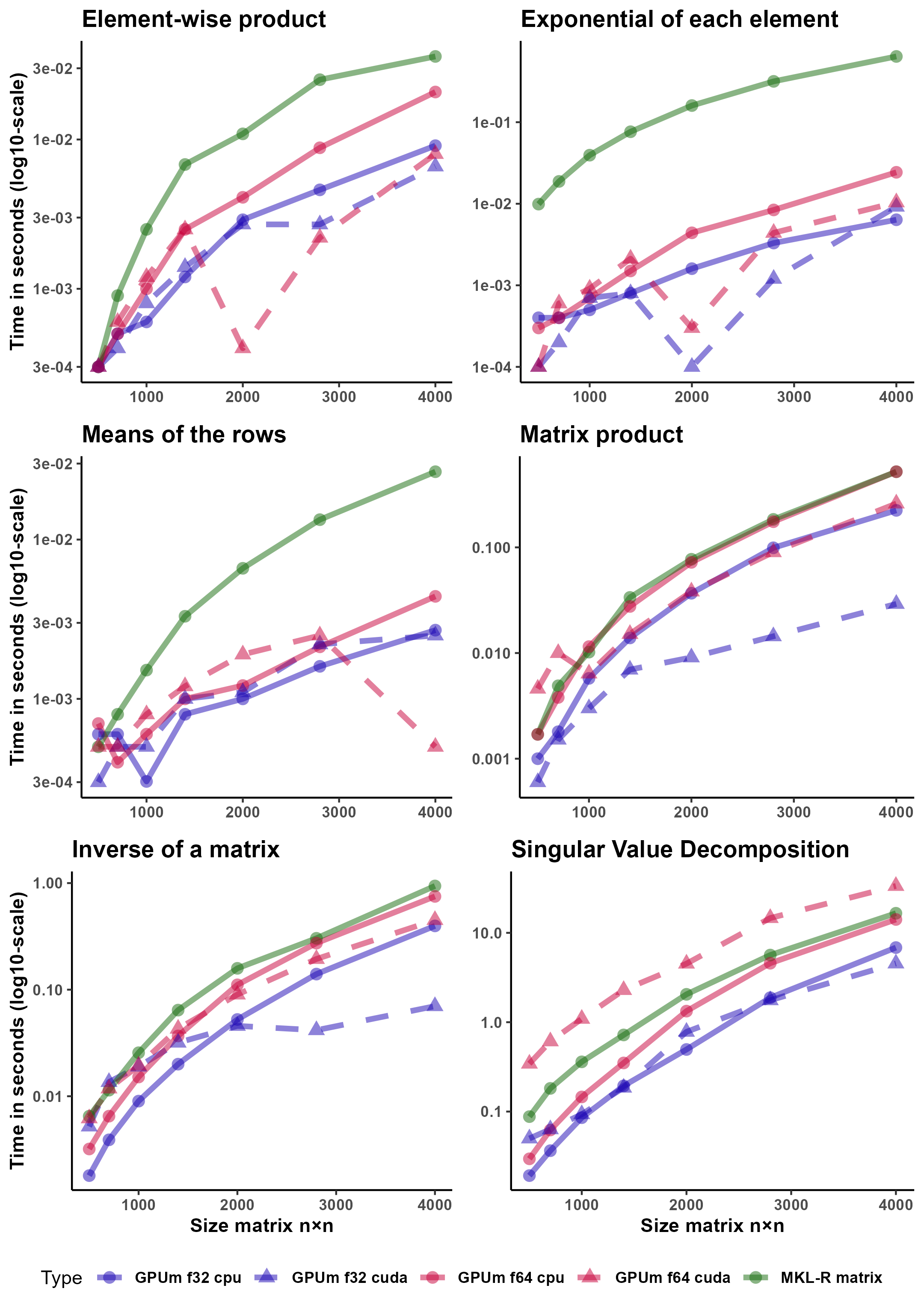
We have compared the computation time for different matrix functions, different precision and running the operations either on the GPU or on the CPU (using both GPUmatrix and plain R).
The functions that we tested are ‘*’ (Hadamard or
element-wise product of matrices), ‘exp’, (exponential of
each element of a matrix), ‘rowMeans’ (means of the rows of
a matrix), ‘%*%’ (standard product of matrices),
‘solve’ (inverse of a matrix) and ‘svd’
(singular value decomposition of a matrix).
These functions were tested on square matrices whose row sizes are 500, 700, 1000, 1400, 2000, 2800 and 4000.
Figure 1 compares the different computational architectures, namely, CPU -standard R matrices running on MKL on FP64-, CPU64 -GPUmatrix matrices computed on the CPU with FP64-, CPU32 -similar to the previous using FP32-, GPU64 -GPUmatrix matrices stored and computed on the GPU with FP64- and GPU32 -identical to the previous using FP32-.
It is important to note that the y-axis is in logarithmic scale. For example, the element-wise product of a matrix on GPU32 is almost two orders of magnitude faster than the same operation on CPU. The results show that the GPU is particularly effective for element-wise operations (Hadamard product, exponential of a matrix). For these operations, it is easier to fully utilize the huge number of cores of a GPU. R-MKL seems to use a single core to perform element-wise operations. The torch implementation is much faster, but not as much as the GPU. rowMeans is also faster on the GPU than on the CPU. In this case, the Torch CPU implementation is on par with the GPU. When the operations become more complex, as in the standard product of matrices and computing the inverse, CPU and GPU (using double precision) are closer to each other. However, GPU32 is still much faster than its CPU32 counterpart. Finally, it is not advisable -in terms of speed- to use the GPU for even more complex operations such as the SVD. In this case, GPU64 is the slowest method. GPU32 hardly stands up to comparison with CPU32.
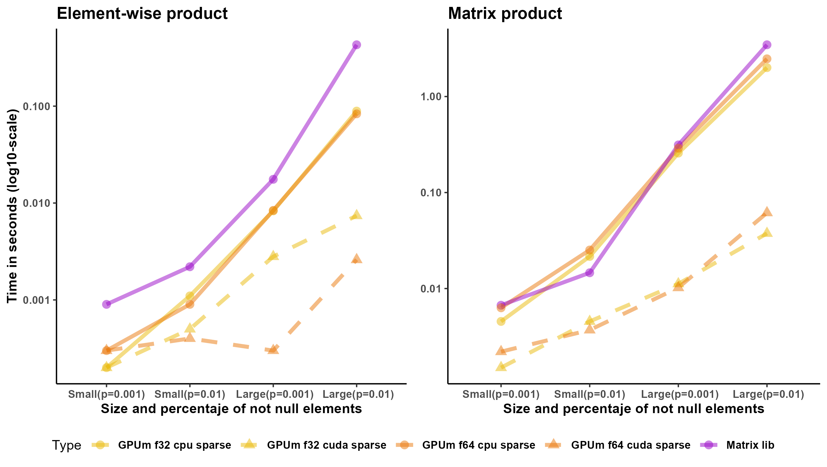
Regarding sparse matrices, Torch or Tensorflow for R have very limited support for them. In many cases, it is necessary to cast the sparse matrix to a full matrix and perform the operations on the full matrix. However, there are two operations that do not require this casting: element-wise multiplication of matrices and multiplication of a sparse matrix and a full matrix. We created four sparse matrices. The size of two of them (small ones) is 2,000 x 2,000. The fraction of nonzero entries is 0.01 and 0.001. The size of the other two (large) is 20,000 x 20,000. The fraction of non-null entries is also 0.01 and 0.001. Figure 2 shows the results for these matrices. As mentioned earlier, the implementation of sparse operations in torch or tensorflow for R is far from perfect, probably, because the only storage mode is “coo” in their respective R packages. Matrix package outperforms either GPU or CPU, even for float32, in all the cases.
GPUmatrix clearly outperforms CPU computation for the element-wise matrix product, since it is not possible to use MKL in these cases.
In all cases, the larger the matrix, the more advantageous it is to compute on the GPU. For the small matrices 500 x 500, the CPU is among the fastest methods for all operations except the exponential computation.
The main advantage of GPUmatrix is its versatility: R code needs only minor changes to adapt it to work in the CPU. We are showing here three statistical applications where its advantages are more apparent.
The non-negative factorization (NMF) of a matrix is an approximate factorization were an initial matrix V is approximated by the product of two matrix W and H so that,
Vm × n ≈ Wm × kHk × n
We have implemented our own non-negative matrix factorization function
(NMFgpumatrix()) using the Lee and Seung multiplicative
update rule.
The rules are
\(\mathbf{W}\_{\[i, j\]}^{n+1} \leftarrow \mathbf{W}\_{\[i, j\]}^n \frac{\left(\mathbf{V}\left(\mathbf{H}^{n+1}\right)^T\right)\_{\[i, j\]}}{\left(\mathbf{W}^n \mathbf{H}^{n+1}\left(\mathbf{H}^{n+1}\right)^T\right)\_{\[i, j\]}}\)
and
\(\mathbf{H}\_{\[i, j\]}^{n+1} \leftarrow \mathbf{H}\_{\[i, j\]}^n \frac{\left(\left(\mathbf{W}^n\right)^T \mathbf{V}\right)\_{\[i, j\]}}{\left(\left(\mathbf{W}^n\right)^T \mathbf{W}^n \mathbf{H}^n\right)\_{\[i, j\]}}\) to update the W and H respectively.
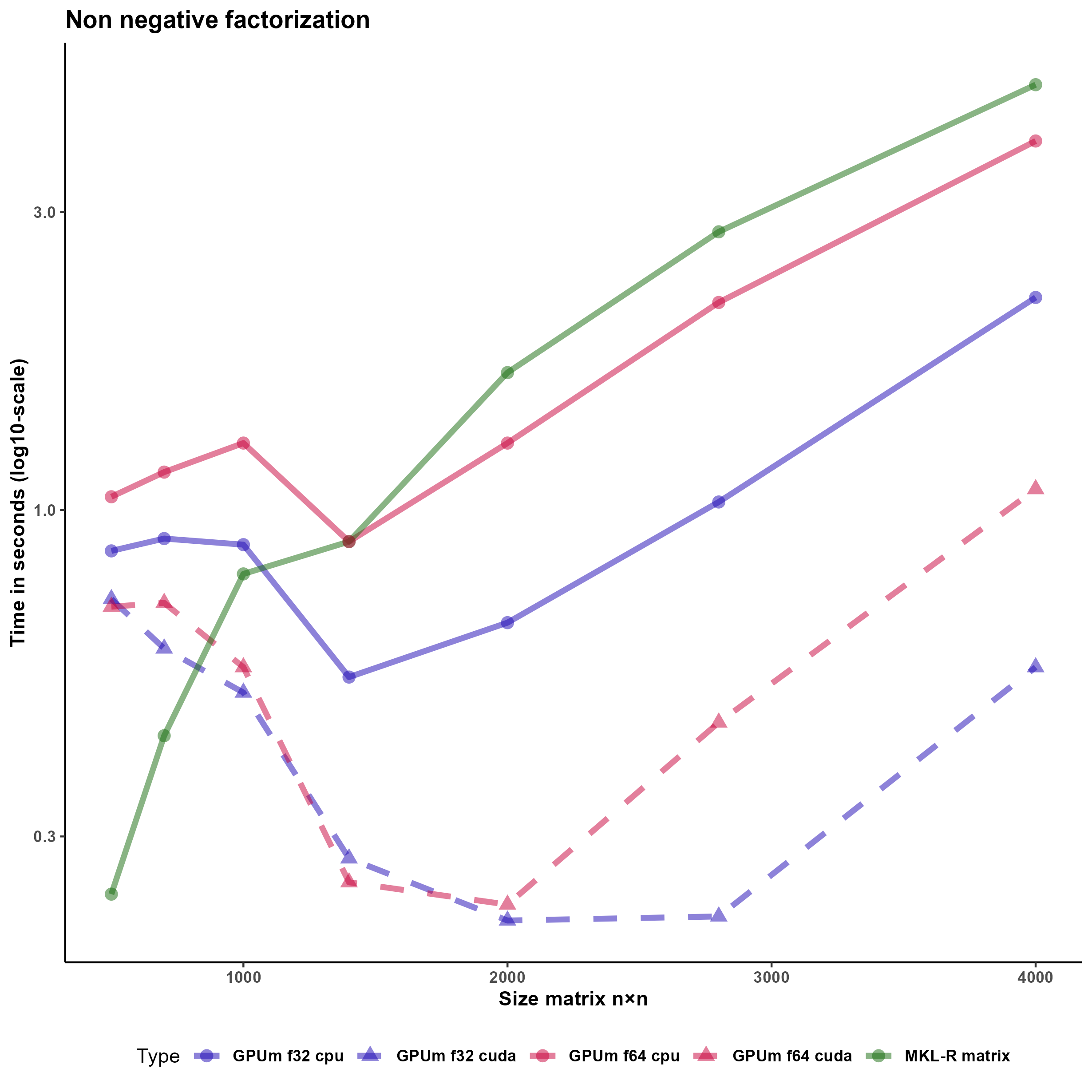
The implemented function is NMFgpumatrix. This function
operates in the same way with basic R matrices as with GPUmatrix
matrices, and it does not require any additional changes beyond
initializing the input matrix as a GPUmatrix. Indeed, the input matrices
W, H, and V can be either gpu.matrix or R base
matrices interchangeably. Figure 3 shows that using GPUmatrix boosts the
performance improvement using both GPU and CPU. This improvement is
especially apparent with float32 matrices.
Logistic regression is a widespread statistical analysis technique
that is the “first to test” method for classification problems where the
outcome is binary. R base implements this analysis in the
glm function. However, glm can be very slow
for big models and, in addition, does not accept sparse coefficient
matrices as input. In this example, we have implemented a logistic
regression solver that accepts as input both dense or sparse
matrices.
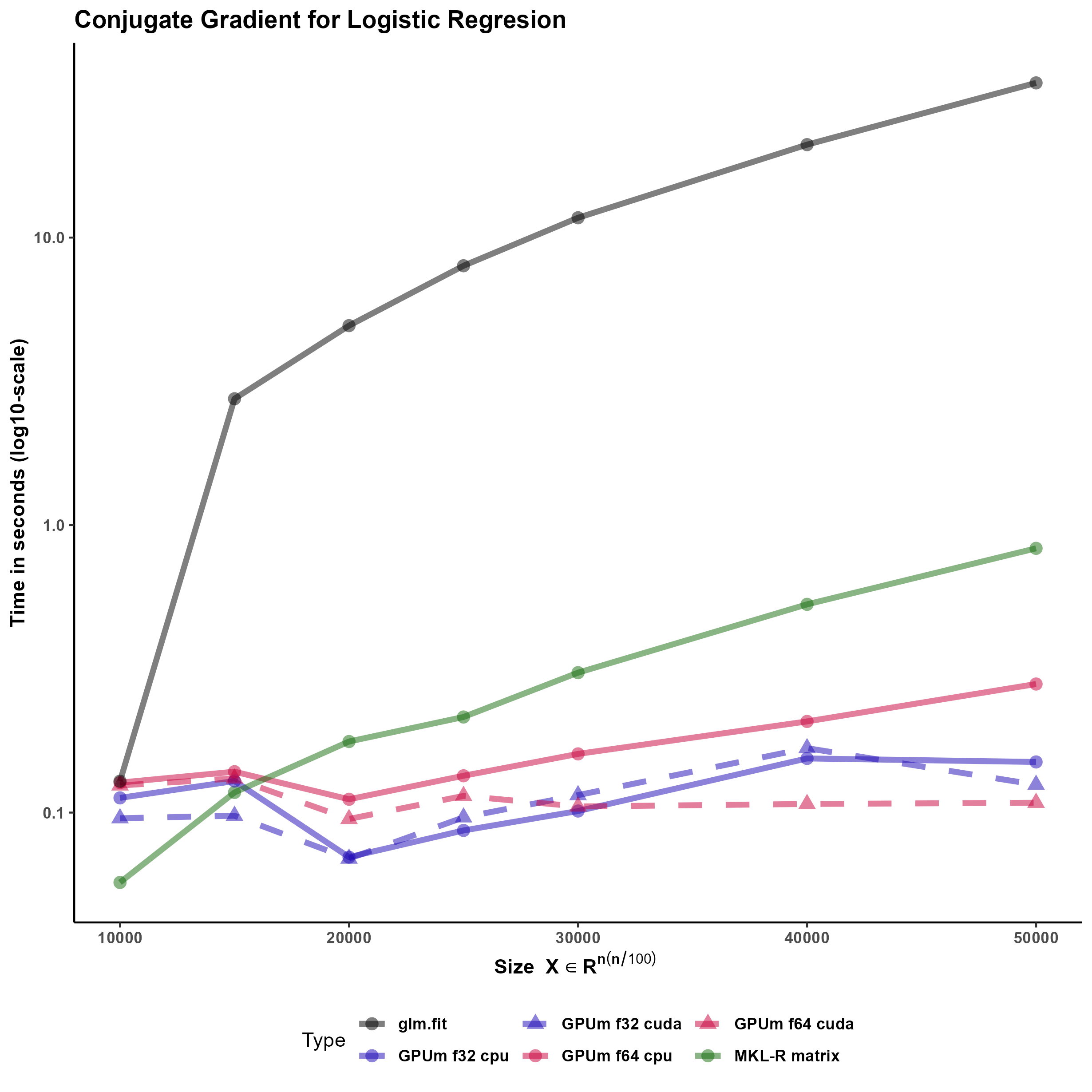
The developed function performs the logistic regression using the Conjugate Gradient method (CG) Figure 4. This method has shown to be very effective for logistic regression of big models (Minka 2003). The code is general enough to accommodate standard R matrices, sparse matrices from the Matrix package and, more interestingly, GPUmatrices from the GPUmatrix package.
We would like to stress several points here. Firstly, the conjugate
gradient is an efficient technique that outperforms glm.fit
in this case. Secondly, this code runs on matrix, Matrix or GPUmatrix
objects without the need of carefully selecting the type of input.
Thirdly, using the GPUmatrix accelerates the computation time two-fold
if compared to standard R (and more than ten fold if compared to
glm.fit function)
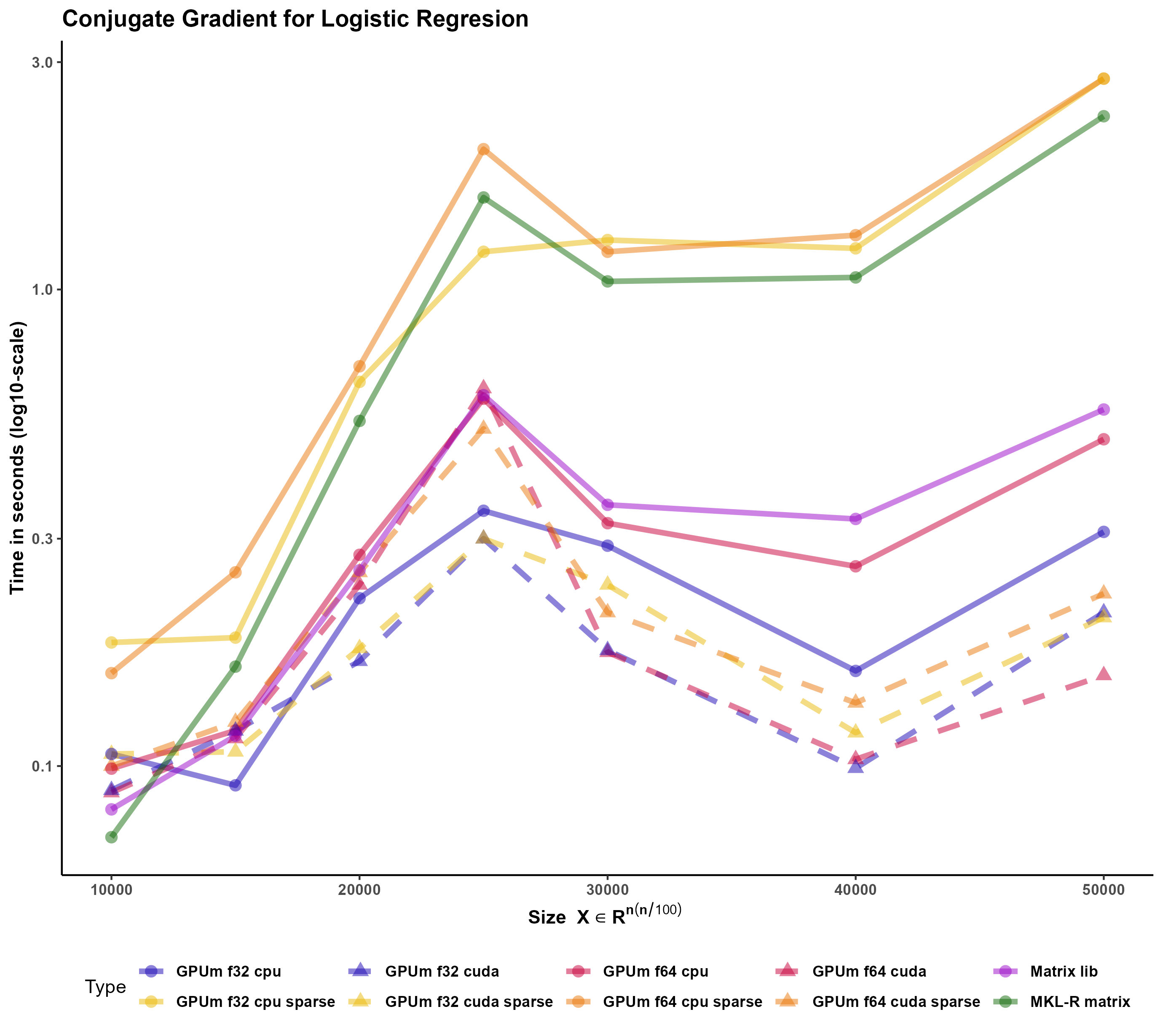
We have tested the function also using a sparse input. In this case, the memory requirements are much smaller. However, there are no advantages in execution time (despite the sparsity is 90 \).
Torch (and Tensorflow) for R only provides a type of sparse matrices: the “coo” coding where each element is described by its position (i and j) and its value. Matrix (and torch and tensorflow for Python) include other storage models (column compressed format, for example) where the matrix computations can be better optimized. It seems that there is still room for improvement in the sparse matrix algebra in Torch for R.
Sparse Matrix -that includes the column compressed form- performs extraordinary well in this case Figure 5. In all the other cases, GPUmatrix in CPU was faster than R-MKL. In this case, despite Matrix is single-threaded, it is roguhly ten times faster than GPUmatrix.
One of the most frequently used functions in R is “glm”, that stands for generalized linear models. In turn, “glm” relies on the “glm.fit”. This function uses the iteratively reweighted least squares algorithm to provide the solution of a generalized linear model. glm.fit, subsequently, calls a C function to do the “hard work” for solving the linear models, including the least squares solution of the intermediate linear systems.
Since glm.fit calls a C function is not easy to develop a “plug-in” substitute using GPUmatrix. Specifically, the qr algorithm in torch or tensorflow for R and in the C function (that is similar to base R) substantially differ: in torch the function returns directly the Q and R matrices whereas the C function called by glm.fit returns a matrix and several auxiliary vectors that can be used to reconstruct the Q and R matrices.
One side-effect of the dependency of base glm on a C function is that, even if R is compiled to use an optimized linear algebra library, the function does not exploit that and the execution time is much longer than expected for this task.
In order to ameliorate this problem, there are other packages (fastlm and speedglm) that mimic the behavior of the base glm. fastlm relies on using multithreaded RcppEigen functions to boost the performance. On the contrary, speedglm is written in plain R and the performance is increased especially if R runs using an optimized BLAS library.
We have used speedglm as starting point for our glm implementation in
the GPU since all the code is written in R and includes no calls to
external functions. Specifically, the most time-consuming task for large
general linear models, is the solution of the intermediate least squares
problems. In the GPUmatrix implementation, we used most of the code of
speed.glm. The only changes are casts on the matrix of the least squares
problem and the corresponding independent term to solve the problem
using the GPU. Timing results of the last section show that
GPUglm outperforms speed.glm for large models.
The following script illustrates how to use the GPUglm
function in toy examples.
# Standard glm

counts <- c(18,17,15,20,10,20,25,13,12)
outcome <- gl(3,1,9)
treatment <- gl(3,3)
glm.D93 <- glm(counts ~ outcome + treatment, family = poisson())
summary(glm.D93)
##
## Call:
## glm(formula = counts ~ outcome + treatment, family = poisson())
##
## Deviance Residuals:
## 1 2 3 4 5 6 7 8
## -0.67125 0.96272 -0.16965 -0.21999 -0.95552 1.04939 0.84715 -0.09167
## 9
## -0.96656
##
## Coefficients:
## Estimate Std. Error z value Pr(>|z|)
## (Intercept) 3.045e+00 1.709e-01 17.815 <2e-16 ***
## outcome2 -4.543e-01 2.022e-01 -2.247 0.0246 *
## outcome3 -2.930e-01 1.927e-01 -1.520 0.1285
## treatment2 1.338e-15 2.000e-01 0.000 1.0000
## treatment3 1.421e-15 2.000e-01 0.000 1.0000
## ---
## Signif. codes: 0 '***' 0.001 '**' 0.01 '*' 0.05 '.' 0.1 ' ' 1
##
## (Dispersion parameter for poisson family taken to be 1)
##
## Null deviance: 10.5814 on 8 degrees of freedom
## Residual deviance: 5.1291 on 4 degrees of freedom
## AIC: 56.761
##
## Number of Fisher Scoring iterations: 4# Using speedglm
library(speedglm)
sglm.D93 <- speedglm(counts ~ outcome + treatment, family = poisson())
summary(sglm.D93)## Generalized Linear Model of class 'speedglm':
##
## Call: speedglm(formula = counts ~ outcome + treatment, family = poisson())
##
## Coefficients:
## ------------------------------------------------------------------
## Estimate Std. Error z value Pr(>|z|)
## (Intercept) 3.045e+00 0.1709 1.781e+01 5.427e-71 ***
## outcome2 -4.543e-01 0.2022 -2.247e+00 2.465e-02 *
## outcome3 -2.930e-01 0.1927 -1.520e+00 1.285e-01
## treatment2 -5.309e-17 0.2000 -2.655e-16 1.000e+00
## treatment3 -2.655e-17 0.2000 -1.327e-16 1.000e+00
##
## -------------------------------------------------------------------
## Signif. codes: 0 '***' 0.001 '**' 0.01 '*' 0.05 '.' 0.1 ' ' 1
##
## ---
## null df: 8; null deviance: 10.58;
## residuals df: 4; residuals deviance: 5.13;
## # obs.: 9; # non-zero weighted obs.: 9;
## AIC: 56.76132; log Likelihood: -23.38066;
## RSS: 5.2; dispersion: 1; iterations: 4;
## rank: 5; max tolerance: 2e-14; convergence: TRUE.# GPU glm
library(GPUmatrix)
gpu.glm.D93 <- GPUglm(counts ~ outcome + treatment, family = poisson())
summary(gpu.glm.D93)## Generalized Linear Model of class 'summary.GPUglm':
##
## Call: glm(formula = ..1, family = ..2, method = "glm.fit.GPU")
##
## Coefficients:
## ------------------------------------------------------------------
## Estimate Std. Error z value Pr(>|z|)
## (Intercept) 3.045e+00 0.1709 1.781e+01 5.427e-71 ***
## outcome2 -4.543e-01 0.2022 -2.247e+00 2.465e-02 *
## outcome3 -2.930e-01 0.1927 -1.520e+00 1.285e-01
## treatment2 2.223e-15 0.2000 1.112e-14 1.000e+00
## treatment3 7.607e-16 0.2000 3.804e-15 1.000e+00
##
## -------------------------------------------------------------------
## Signif. codes: 0 '***' 0.001 '**' 0.01 '*' 0.05 '.' 0.1 ' ' 1
##
## ---
## null df: 8; null deviance: 10.58;
## residuals df: 4; residuals deviance: 5.13;
## # obs.: 9; # non-zero weighted obs.: 9;
## AIC: 56.76132; log Likelihood: -23.38066;
## RSS: 5.2; dispersion: 1; iterations: 4;
## rank: 5; max tolerance: 2.04e-14; convergence: TRUE.Results are identical in this test.
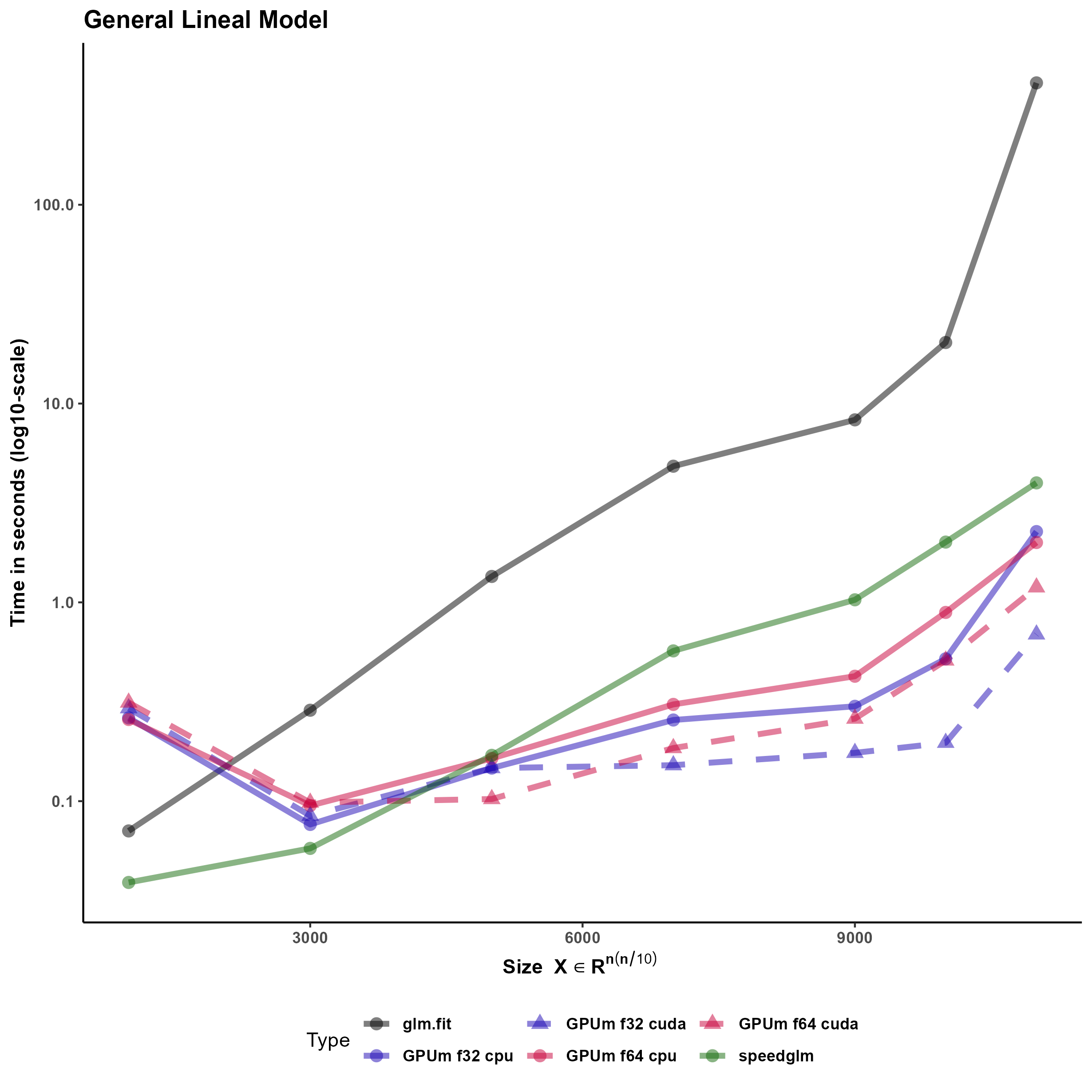
Figure 6 compares the timing of the implementation using speedglm, glm and the implementation of glm in GPUmatrix.
Bates D, Maechler M, Jagan M (2022). Matrix: Sparse and Dense Matrix Classes and Methods. R package version 1.5-3, https://CRAN.R-project.org/package=Matrix.
Schmidt D (2022). “float: 32-Bit Floats.” R package version 0.3-0, https://cran.r-project.org/package=float.
Falbel D, Luraschi J (2022). torch: Tensors and Neural Networks with ‘GPU’ Acceleration. R package version 0.9.0, https://CRAN.R-project.org/package=torch.
Allaire J, Tang Y (2022). tensorflow: R Interface to ‘TensorFlow’. R package version 2.11.0, https://CRAN.R-project.org/package=tensorflow.
Minka, Thomas P. 2003. “A Comparison of Numerical Optimizers for Logistic Regression.” https://tminka.github.io/papers/logreg/minka-logreg.pdf.