
![]()
![]()
Contributors: Yongqi Zhong, Ashley Naimi, Gabriel Conzuelo, Edward Kennedy
Augmented inverse probability weighting (AIPW) is a doubly robust
estimator for causal inference. The AIPW package is
designed for estimating the average treatment effect of a binary
exposure on risk difference (RD), risk ratio (RR) and odds ratio (OR)
scales with user-defined stacked machine learning algorithms (SuperLearner
or sl3). Users need to
examine causal assumptions (e.g., consistency) before using this
package.
If you find this package is helpful, please consider to cite:
@article{zhong_aipw_2021,
    author = {Zhong, Yongqi and Kennedy, Edward H and Bodnar, Lisa M and Naimi, Ashley I},
    title = {AIPW: An R Package for Augmented Inverse Probability Weighted Estimation of Average Causal Effects},
    journal = {American Journal of Epidemiology},
    year = {2021},
    month = {07},
    issn = {0002-9262},
    doi = {10.1093/aje/kwab207},
    url = {https://doi.org/10.1093/aje/kwab207},
}The major new feature introduced is the Repeated class,
which allows for repeated cross-fitting procedures to mitigate
randomness due to data splits in machine learning-based estimation as
suggested by Chernozhukov et al. (2018). This feature: - Enables running
the cross-fitting procedure multiple times to produce more stable
estimates - Provides methods to summarize results using median-based
approaches - Supports parallelization with future.apply -
Includes visualization of estimate distributions across repetitions -
See the Repeated
Cross-fitting vignette for more details
remotes::install_github("yqzhong7/AIPW@aje_version")install.packages("AIPW")install.packages("remotes")
remotes::install_github("yqzhong7/AIPW")* CRAN version only supports SuperLearner and tmle. New
GitHub versions (after v0.6.3.1) no longer support sl3 and tmle3. If you
are still interested in using the version with sl3 and tmle3 support,
please install
remotes::install_github("yqzhong7/AIPW@aje_version")
Please install the Github version (master branch) if you choose to
use sl3 and tmle3.
set.seed(888)
data("eager_sim_obs")
outcome <- eager_sim_obs$sim_Y
exposure <- eager_sim_obs$sim_A
#covariates for both outcome model (Q) and exposure model (g)
covariates <- as.matrix(eager_sim_obs[-1:-2])

# covariates <- c(rbinom(N,1,0.4)) #a vector of a single covariate is also supportedAIPW class: method chaining from
R6class)library(AIPW)
library(SuperLearner)
#> Loading required package: nnls
#> Loading required package: gam
#> Loading required package: splines
#> Loading required package: foreach
#> Loaded gam 1.20.2
#> Super Learner
#> Version: 2.0-28
#> Package created on 2021-05-04
library(ggplot2)
AIPW_SL <- AIPW$new(Y = outcome,
A = exposure,
W = covariates,
Q.SL.library = c("SL.mean","SL.glm"),
g.SL.library = c("SL.mean","SL.glm"),
k_split = 3,
verbose=FALSE)$
fit()$
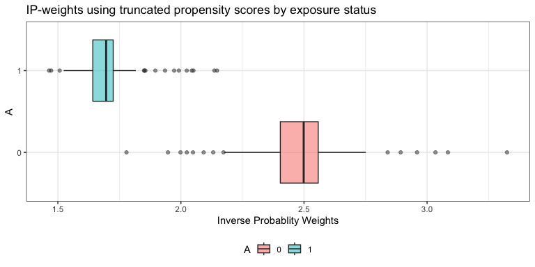
#Default truncation
summary(g.bound = 0.025)$
plot.p_score()$
plot.ip_weights()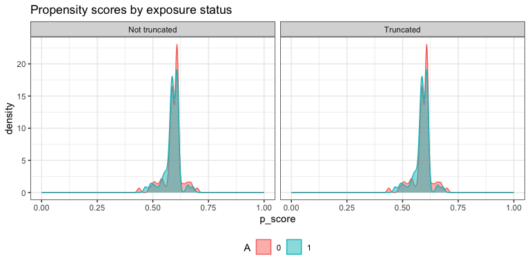
To see the results, set verbose = TRUE(default) or:
print(AIPW_SL$result, digits = 2)
#>                  Estimate    SE 95% LCL 95% UCL   N
#> Risk of Exposure     0.44 0.046  0.3528    0.53 118
#> Risk of Control      0.31 0.051  0.2061    0.41  82
#> Risk Difference      0.14 0.068  0.0048    0.27 200
#> Risk Ratio           1.45 0.191  0.9974    2.11 200
#> Odds Ratio           1.81 0.295  1.0144    3.22 200
To obtain average treatment effect among the treated/controls
(ATT/ATC), statified_fit() must be used:
AIPW_SL_att <- AIPW$new(Y = outcome,
                    A = exposure,
                    W = covariates,
                    Q.SL.library = c("SL.mean","SL.glm"),
                    g.SL.library = c("SL.mean","SL.glm"),
                    k_split = 3,
                    verbose=T)
suppressWarnings({
  AIPW_SL_att$stratified_fit()$summary()
})
#> Done!
#>                     Estimate     SE  95% LCL 95% UCL   N
#> Risk of Exposure      0.4352 0.0467  0.34362   0.527 118
#> Risk of Control       0.3244 0.0513  0.22385   0.425  82
#> Risk Difference       0.1108 0.0684 -0.02320   0.245 200
#> Risk Ratio            1.3416 0.1858  0.93210   1.931 200
#> Odds Ratio            1.6048 0.2927  0.90429   2.848 200
#> ATT Risk Difference   0.0991 0.0880 -0.07339   0.272 200
#> ATC Risk Difference   0.1148 0.0634 -0.00946   0.239 200
You can also use the aipw_wrapper() to wrap
new(), fit() and summary()
together (also support method chaining):
AIPW_SL <- aipw_wrapper(Y = outcome,
                        A = exposure,
                        W = covariates,
                        Q.SL.library = c("SL.mean","SL.glm"),
                        g.SL.library = c("SL.mean","SL.glm"),
                        k_split = 3,
                        verbose=TRUE,
stratified_fit=F)$plot.p_score()$plot.ip_weights()The Repeated class allows for repeated cross-fitting
procedures to mitigate randomness due to data splits. This approach is
recommended in machine learning-based estimation as suggested by
Chernozhukov et al. (2018).
library(SuperLearner)
library(ggplot2)

# First create a regular AIPW object
aipw_obj <- AIPW$new(Y = outcome,
                     A = exposure,
                     W = covariates,
                     Q.SL.library = c("SL.mean","SL.glm"),
                     g.SL.library = c("SL.mean","SL.glm"),
                     k_split = 3,
                     verbose = FALSE)

# Create a repeated fitting object from the AIPW object
repeated_aipw <- Repeated$new(aipw_obj)

# Perform repeated fitting 20 times
repeated_aipw$repfit(num_reps = 20, stratified = FALSE)

# Summarize results using median-based methods
repeated_aipw$summary_median()

# You can also visualize the distribution of estimates across repetitions
estimates_df <- repeated_aipw$repeated_estimates
ggplot(estimates_df, aes(x = Estimate, fill = Estimand)) +
  geom_density(alpha = 0.5) +
  theme_minimal() +
  labs(title = "Distribution of Estimates Across Repeated Fittings",
       subtitle = "Based on 20 repetitions",
       x = "Estimate Value",
       y = "Density")
Setting stratified = TRUE in the repfit()
function will use the stratified fitting procedure for each
repetition:
# Using stratified fitting
repeated_aipw_strat <- Repeated$new(aipw_obj)
repeated_aipw_strat$repfit(num_reps = 20, stratified = TRUE)
repeated_aipw_strat$summary_median()
Note that the Repeated class also supports
parallelization with future.apply as described below.
future.apply and progress bar with
progressrIn default setting, the AIPW$fit() method will be run
sequentially. The current version of AIPW package supports parallel
processing implemented by future.apply
package under the future framework.
Simply use future::plan() to enable parallelization and
set.seed() to take care of the random number generation
(RNG) problem:
###Additional steps for parallel processing###
# install.packages("future.apply")
library(future.apply)
#> Loading required package: future
future::plan(multiprocess, workers=2, gc=T)
#> Warning: Strategy 'multiprocess' is deprecated in future (>= 1.20.0)
#> [2020-10-30]. Instead, explicitly specify either 'multisession' (recommended) or
#> 'multicore'. In the current R session, 'multiprocess' equals 'multisession'.
#> Warning in supportsMulticoreAndRStudio(...): [ONE-TIME WARNING] Forked
#> processing ('multicore') is not supported when running R from RStudio
#> because it is considered unstable. For more details, how to control forked
#> processing or not, and how to silence this warning in future R sessions, see ?
#> parallelly::supportsMulticore
set.seed(888)

###Same procedure for AIPW as described above###
AIPW_SL <- AIPW$new(Y = outcome,
                    A = exposure,
                    W = covariates,
                    Q.SL.library = c("SL.mean","SL.glm"),
                    g.SL.library = c("SL.mean","SL.glm"),
                    k_split = 3,
                    verbose=TRUE)$fit()$summary()
#> Done!
#>                  Estimate     SE 95% LCL 95% UCL   N
#> Risk of Exposure    0.443 0.0462 0.35284   0.534 118
#> Risk of Control     0.306 0.0510 0.20607   0.406  82
#> Risk Difference     0.137 0.0677 0.00482   0.270 200
#> Risk Ratio          1.449 0.1906 0.99741   2.106 200
#> Odds Ratio          1.807 0.2946 1.01442   3.219 200
Progress bar that supports parallel processing is available in the
AIPW$fit() method through the API from progressr
package:
library(progressr)
#define the type of progress bar
handlers("progress")
#reporting through progressr::with_progress() which is embedded in the AIPW$fit() method
with_progress({
  AIPW_SL <- AIPW$new(Y = outcome,
                    A = exposure,
                    W = covariates,
                    Q.SL.library = c("SL.mean","SL.glm"),
                    g.SL.library = c("SL.mean","SL.glm"),
                    k_split = 3,
                    verbose=FALSE)$fit()$summary()
})
#also available for the wrapper
with_progress({
  AIPW_SL <- aipw_wrapper(Y = outcome,
                        A = exposure,
                        W = covariates,
                        Q.SL.library = c("SL.mean","SL.glm"),
                        g.SL.library = c("SL.mean","SL.glm"),
                        k_split = 3,
                        verbose=FALSE)
})tmle/tmle3 fitted object as input
(AIPW_tmle class)AIPW_tmle class is designed for using
tmle/tmle3 fitted object as input
tmlerequire(tmle)
#> Loading required package: tmle
#> Loading required package: glmnet
#> Loading required package: Matrix
#> Loaded glmnet 4.1-6
#> Welcome to the tmle package, version 1.5.0-1.1
#>
#> Major changes since v1.3.x. Use tmleNews() to see details on changes and bug fixes
require(SuperLearner)
tmle_fit <- tmle(Y = as.vector(outcome), A = as.vector(exposure),W = covariates,
Q.SL.library=c("SL.mean","SL.glm"),
g.SL.library=c("SL.mean","SL.glm"),
family="binomial")
tmle_fit
#> Additive Effect
#> Parameter Estimate: 0.12795
#> Estimated Variance: 0.0043047
#> p-value: 0.051161
#> 95% Conf Interval: (-0.00064797, 0.25654)
#>
#> Additive Effect among the Treated
#> Parameter Estimate: 0.13118
#> Estimated Variance: 0.0045329
#> p-value: 0.051365
#> 95% Conf Interval: (-0.00077957, 0.26314)
#>
#> Additive Effect among the Controls
#> Parameter Estimate: 0.12446
#> Estimated Variance: 0.00414
#> p-value: 0.05307
#> 95% Conf Interval: (-0.0016502, 0.25057)
#>
#> Relative Risk
#> Parameter Estimate: 1.4093
#> p-value: 0.064957
#> 95% Conf Interval: (0.97895, 2.0288)
#>
#> log(RR): 0.34308
#> variance(log(RR)): 0.034558
#>
#> Odds Ratio
#> Parameter Estimate: 1.7316
#> p-value: 0.057367
#> 95% Conf Interval: (0.98296, 3.0504)
#>
#> log(OR): 0.54905
#> variance(log(OR)): 0.083461
#extract fitted tmle object to AIPW
AIPW_tmle$
new(A=exposure,Y=outcome,tmle_fit = tmle_fit,verbose = TRUE)$
summary(g.bound=0.025)
#> Cross-fitting is supported only within the outcome model from a fitted tmle object (with cvQinit = TRUE)
#> Estimate SE 95% LCL 95% UCL N
#> Risk of Exposure 0.441 0.0447 0.352877 0.528 118
#> Risk of Control 0.313 0.0503 0.214003 0.411 82
#> Risk Difference 0.128 0.0656 -0.000648 0.257 200
#> Risk Ratio 1.409 0.1814 0.987632 2.011 200
#> Odds Ratio 1.732 0.2814 0.997604 3.006 200tmle3__New GitHub versions (after v0.6.3.1) no longer support sl3 and tmle3. If you are still interested in using the version with sl3 and tmle3 support, please install `remotes::install_github(“yqzhong7/AIPW@aje_version”)__
remotes::install_github("yqzhong7/AIPW@aje_version")
library(sl3)
library(tmle3)
node_list <- list(A = "sim_A",Y = "sim_Y",W = colnames(eager_sim_obs)[-1:-2])
or_spec <- tmle_OR(baseline_level = "0",contrast_level = "1")
tmle_task <- or_spec$make_tmle_task(eager_sim_obs,node_list)
lrnr_glm <- make_learner(Lrnr_glm)
lrnr_mean <- make_learner(Lrnr_mean)
sl <- Lrnr_sl$new(learners = list(lrnr_glm,lrnr_mean))
learner_list <- list(A = sl, Y = sl)
tmle3_fit <- tmle3(or_spec, data=eager_sim_obs, node_list, learner_list)

# parse tmle3_fit into AIPW_tmle class
AIPW_tmle$
  new(A=eager_sim_obs$sim_A,Y=eager_sim_obs$sim_Y,tmle_fit = tmle3_fit,verbose = TRUE)$
summary()Robins JM, Rotnitzky A (1995). Semiparametric efficiency in multivariate regression models with missing data. Journal of the American Statistical Association.
Chernozhukov V, Chetverikov V, Demirer M, et al (2018). Double/debiased machine learning for treatment and structural parameters. The Econometrics Journal.
Kennedy EH, Sjolander A, Small DS (2015). Semiparametric causal inference in matched cohort studies. Biometrika.
Pearl, J., 2009. Causality. Cambridge university press.